The normal distribution Normal distribution Normal distribution Continuous
")
The normal distribution (정규분포)
 – Continuous probability distribution (연속확률분포 ) – Continuous")
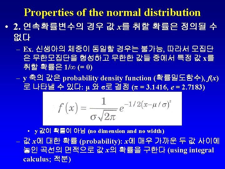
Normal distribution • Normal distribution (정규분포) – Continuous probability distribution (연속확률분포 ) – Continuous variables (연속변수)이 이러한 분포를 보임 (ex. heights, weights, 생산량 등) – 값의 범위가 충분히 클 경우 많은 discrete variables (불연속변수, 이산변수)도 정규분포를 따른다 – 많은 경우 확률을 쉽게 결정하기 위해 normal distribution을 이용한다 – 따라서 normal distribution은 많은 통계처리 (ttest, ANOVA, regression analysis)의 기초가 된다

Normal distribution and its properties • Continuous measurement variables에서는 특정 범 위 내의 어떤 값이든 추정할 수 있다 • 따라서 sample size가 아주 커질 경우 histogram은 smooth curve가 된다 • 이러한 곡선을 나타내는 probability distribution을 normal probability distribution (정규확률분포)라 한다 • 좌우대칭의 종모양의 곡선 – Population mean: μ – 좌우 무한대 (±∞)로 뻗어나가면 x축에 접근
 • 1. The distribution은 mean (μ)과 standard")
Properties of the normal distribution (정규분포의 특성) • 1. The distribution은 mean (μ)과 standard deviation (σ)로 정의된 다 – x 축 상의 위치는 mean (μ) 에 의해, – 곡선의 퍼짐은 standard deviation (σ)에 의해 결정 된다 – 이러한 parameters의 값 은 무한하므로 무한한 종 류의 normal distribution A, B: different means, same variance B, C: same mean, different variances
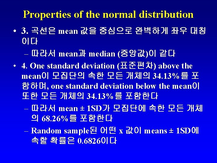

Properties of the normal distribution • 4. mean± 2 SD는 95. 46%를 the mean ± 3 SD는 99. 73%를 포함한다 • Normal curve가 차지하는 총면적은 1이다

The standard normal distribution and Z scores • Ex. 6. 1: 부산대학의 일반생물학을 수강하는 학생의 키를 조사 (n = 414) – 전체학생의 키를 측정 – Mean height = 166. 8 cm, standard deviation = 6. 4 cm – This mean과 standard deviation은 parameters (모수) or statistics (통계치)? ? • Parameters • Mean height (μ) = 166. 8 cm, standard deviation (σ) = 6. 4 cm – Question 1: 키가 170 cm 인 학생의 z score는? • z = (x – μ)/σ = (170 – 166. 8)/6. 4 = 0. 5 – Question 2: 170 cm 이하의 키를 가진 학생은 몇 %인가? (Table A. 1을 이용)

The standard normal distribution and Z scores • The shaded area of the curve는 mean 과 z value 사이에 해당하 는 standard normal distribution의 proportion을 의미한다 – In Table A. 1, z score 0. 50에 해당하는 값: 0. 1915 • Mean과 z score 0. 5 사이에 해당하는 proportion이 0. 1915라는 의미 • 166. 8 cm – 170 cm: 전체학생의 19. 15% • 정규분포는 완전한 좌우대칭, 따라서 mean 이하에 해당하는 proportion 이 0. 5 (166. 8 cm 이하인 학생은 전체의 50%) – 따라서 170 cm 이하의 학생의 proportion? • 0. 1915 + 0. 5 = 0. 6915 (69. 15%)

The standard normal distribution and z scores • Question 3: 163. 6 cm 보다 작은 학생들의 비율은?
/σ =")
The standard normal distribution and Z scores • z = (x – μ)/σ = (163. 6 – 166. 8)/6. 4 = -0. 5 • Standard normal distribution은 완전한 좌우대칭 • 따라서 mean에서 + 0. 5 사이의 proportion과 mean 에서 -0. 5 사이의 proportion이 같다 • 따라서 mean 과 z score -0. 5 사이의 proportion: 0. 1915 – Mean (166. 8 cm)과 163. 6 cm 사이에 해당하는 학생의 proportion: 0. 1915 • z score -0. 5 이하에 해당하는proportion? – 0. 5000 – 0. 1915 = 0. 3085 (30. 85%) – 약 31%의 학생이 163. 6 cm 이하

The standard normal distribution and z scores • Question 4: 160 cm – 170 cm 사이의 학생들 의 비율은?

The standard normal distribution and Z scores • z score for 160 cm = (x – μ)/σ = (160 – 166. 8)/6. 4 = -1. 063 – According to Table A. 1, 1. 06 = 0. 3554 – For 1. 063: 0. 3554 + {(0. 3577 – 0. 3554) × 0. 3} = 0. 35609 • z score for 170 cm = (x – μ)/σ = (170 – 166. 8)/6. 4 = 0. 5 – According to Table A. 1, 0. 5 = 0. 1915 • 따라서 160 -170 cm에 해당하는 proportion? – 0. 35609 + 0. 1915 = 0. 54759 (54. 759%) – 약 55%의 학생이 160 cm 에서 170 cm 사이 – Random sample 할 경우 160 -170 cm 사이의 학생이 선택될 확률이 55%
를")
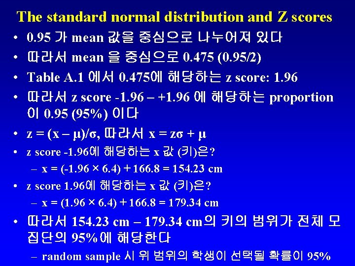
The standard normal distribution and Z scores • Question 5: 모집단의 0. 95 (95%)를 포함하는 키의 범위를 구하라. – Mean height = 166. 8 cm, standard deviation = 6. 4 cm – z = (x – μ)/ σ

Exercises • Question 1: 송사리의 크기 – The mean length of the population: 34. 29 mm – The standard deviation: 5. 49 mm • 1. 이 population에서 50 mm 이상의 개체가 채집될 확률은?

Exercises • Question 1: 송사리의 크기 – The mean length of the population: 34. 29 mm – The standard deviation: 5. 49 mm • 1. 이 population에서 50 mm 이상의 개체가 채집될 확률은? • z score for 50 mm: z = (50 – 34. 29)/5. 49 = 2. 86 • In Table A. 1, area for z score 2. 86: 0. 4979 • 따라서 50 mm 이상일 확률은: 0. 5 – 0. 4979 = 0. 0021
 • 대부분의 statistical tests는 variables (변수)이 normal distribution을 하고")
Testing for normality (정규성 검정) • 대부분의 statistical tests는 variables (변수)이 normal distribution을 하고 있다는 것을 가정한다 – 적어도 approximately (근사적) normally distributed • 많은 biological variables는 normally distributed • 그러나 normal distribution을 하고 있다는 것을 객관 적인 방법으로 보여주어야 한다 – Normality test (정규성 검정): data의 분포가 정규 분포를 따르는지를 검정 – 한가지 방법: frequency distribution을 분석함으로 써 normal distribution을 하고 있다는 것을 보여줄 수 있다
, n = 148 • Histogram")
Testing for normality • Ex. 남자의 키 (in cm), n = 148 • Histogram using a class interval of 2 cm • Histogram이 more or less bell-shaped • 그리고 전체적인 모양이 normal distribution처럼 보임 • 그러나 더 나은 방법이 필요

Testing for normality • Probability plot을 이용하면 normal distribution을 더 명확히 알 수 있다 • Probability plot – y-axis: 누적 frequency (누적빈도) – x-axis: original measurement variable – Normal distribution을 할 경우 straight line – 손으로 plotting 하는 것이 쉽지 않음 – Normality을 검정하는 많은 통계 program이 있음

Testing for normality • Figure 6. 8: Anderson Darling test를 이용 • p > 0. 05 보다 클 경우 normal distribution • 이 경우 p = 0. 201, 따라서 normal distribution

Parametric and nonparametric statistics • 모수검정 과 비모수검정 • 주로 사용하는 대부분의 통계처리들은 몇 가지 중요한 가정 (assumptions)을 만족해야 함 • 1. the variable is at least approximately normally distributed • 2. the variable is measured on an interval or ratio scale • 위 두 조건을 만족할 경우 – Parametric test를 적용할 수 있다 – Parametric test는 normal distribution을 이용하므로 • 위 조건을 만족하지 못할 경우 – Nonparametric test를 사용해야 함 • Ordinal scale로 측정된 data에도 비모수검정이 유용
 of the binominal distribution • 이항분포에서 k (number of case)가 아주")
Normal approximation (정규근사) of the binominal distribution • 이항분포에서 k (number of case)가 아주 클 경 우 확률계산이 tedious • Normal distribution으로 해결 가능 • k가 상당히 크고 p가 0 or 1에 너무 가깝지 않 을 경우 binominal distribution은 normal distribution과 유사하게 된다 • Fairly large? ? – k × p and k × q, 둘 다 5이상일 경우
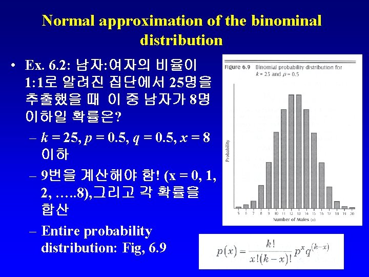

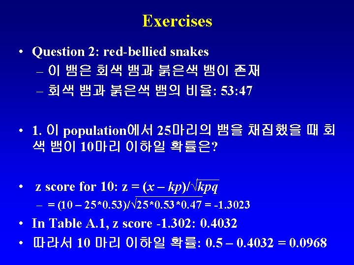
Normal approximation of the binominal distribution • Both k × p and k × q: 12. 5 • Normal distribution을 이용할 수 있다 • Binomial variables – Mean (μ) = kp; σ = √kpq • • μ = 25 × 0. 5 = 12. 5, σ = √kpq = √ 25 × 0. 5 = 2. 5 8의 z score: z = (8 – 12. 5)/2. 5 = -1. 8 In Table A. 1: z score 1. 8 = 0. 4641 8이하의 확률: 0. 5 – 0. 4641 = 0. 0359 Computer program으로 계산한 값: 0. 0322: 비슷함 z = (x – kp)/ √kpq
- Slides: 31