The Normal Distribution Chapter 2 The Normal Distribution

The Normal Distribution Chapter 2

The Normal Distribution The assumption that something is “Normal” is one of the most important things in Statistics. Think of a list of numbers that has low values, high values, and values in the middle. If you have LOTS of these types of numbers then they MIGHT follow a “Normal Distribution” A good example might be the height of ALL women in the United States. This would be a list of millions of numbers. They would all average to a certain height(the mean). There would be some very tall women and some very short women, because there are SO MANY women in the United States, this data would follow a Normal Distribution. Other things that might follow a Normal Distribution: test scores for ALL of tests in AP Stats, the time it takes you to get to school for all of the school days this year, shoes sizes for men, IQ scores, the number of times that you blink each day, …. . etc.

CAUTION!! Not all data follows a Normal Distribution Data with outliers or skewness may not be Normally distributed Large samples will be closer to a Normal distribution than small samples Real life data is almost NEVER EXACTLY NORMAL.

The Normal Distribution The area under the curve represents 100% of the observations/data.

The Normal Distribution The center of the curve is the mean, median, and the 50 th percentile.

The Empirical Rule 68, 95, 99. 7 68% of the data is within 1 St. Dev of the mean 95% of the data is within 2 St. Dev of the mean 99. 7% of the data is within 3 St. Dev of the mean

The mean and standard deviation describe a Normal Distribution. We write it like this: Describing a Normal Distribution

Let’s say that the mean height for all men in Garden Grove is 68 inches with a standard deviation of 4 inches. We would need to write our description like this: Describing a Normal Distribution

Let’s say that the mean time it takes Mr. Pines to walk to the office each day is 242 seconds with a standard deviation of 11 seconds. We would need to write our description like this: Describing a Normal Distribution

Sample Test Scores for a typical math class. Draw a Normal Curve with Mean μ = 70 and Standard Deviation σ = 10 μ 40 50 60 70 80 90 100 What percent of the data was less than 80? What percent of the data was between 50 and 90? What score was at the 50 th percentile? What score would be the 16 th percentile?

Draw a Normal Curve with Mean μ = 70 and Standard Deviation σ = 10 μ 40 50 60 70 80 90 100 What percent of the data was less than 80? about 84% What percent of the data was between 50 and 90? about 95% What score was at the 50 th percentile? 70 What score would be the 16 th percentile? 60

Z - Scores A Z-score is the number of Standard Deviations above or below the mean You can be asked to find any of the 4 pieces in the above equation. If given a percentage you need to use the inv. Norm function on your calculator to get the Z -score.

Assume a Normal Distribution with a Mean μ = 70 and Standard Deviation σ = 10. Calculate the Z-score a score of 83. Z = 1. 3 which means that a score of 83 is 1. 3 standard deviations above the mean.

Scores from Miss Turrys quiz on Dinosaurs. 0 012 1 2248 2 1134599 3 00036 4 457 5 0 1) Calculate the mean and standard deviation. 2) Interpret the meaning of the standard deviation in this context.

Scores from Miss Turrys quiz on Dinosaurs. 0 012 1 2248 2 1134599 3 00036 4 457 5 0 3) Peppa earned a 45. Calculate and interpret her z-score. 4) George earned a 2. Calculate and interpret his z-score.

Scores from Miss Turry’s quiz on Dinosaurs. 0 012 1 2248 2 1134599 3 00036 4 457 5 0 5) The scores on Miss Turry’s next quiz had a mean of 32 and a standard deviation of 6. 5. Peppa earned a 47 on this quiz. On which quiz did she perform better relative to the rest of the class? Explain

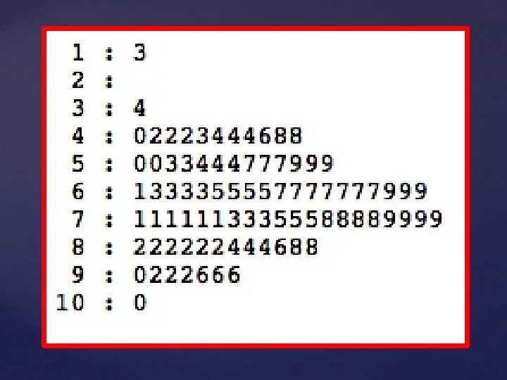
Ch 5 Test Scores n = 85

n = 85 Based on the mean and median, it appears that the distribution of test scores are approximately Normal.

n = 85

Sketch a Normal Curve using the mean and standard deviation above. Compare the distribution of Ch 5 test scores to the Empirical Rule.

Standard Normal Curve N(0, 1)

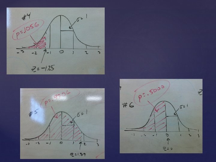
Find the percentile for the following Z-scores 1. z = 2. 34 2. z = -. 34 Use the Yellow Table. 3. z = -. 27 4. z = -1. 25 5. z = 1. 89 6. z = 0 Use your

Given the percentile, find the Z-score 1. p =. 2673 2. p =. 1238 Use the Yellow Table. 3. p =. 9472 4. p =. 5632 5. p =. 2167 6. p =. 7654 Use your

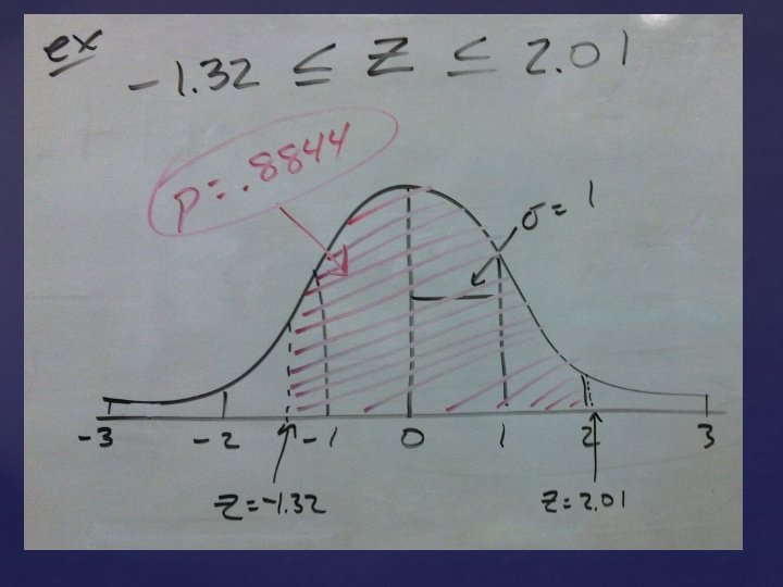
Sketch the curve, find the percent/probability and shade. 1. z > 1. 34 2. z < 2. 15 Use the Yellow Table. 3. z < -2. 34 4. z > 2. 90 5. z < 1. 34 6. z > -. 28 Use your normalcdf(

Sketch the curve, find the z-score. 1. p =. 6348 2. p =. 22 Use the Yellow Table. 3. 75 th percentile or 4. Top 10 percentile Use your inv. Norm

Great White Sharks

Lengths of 44 Great White Sharks Find the Mean and Standard Deviation 18. 7 12. 3 18. 6 16. 4 15. 7 18. 3 14. 6 15. 8 14. 9 17. 6 12. 1 16. 4 16. 7 17. 8 16. 2 12. 6 17. 8 13. 8 12. 2 15. 2 14. 7 12. 4 13. 2 15. 8 14. 3 16. 6 9. 4 18. 2 13. 6 15. 3 16. 1 13. 5 19. 1 16. 2 22. 8 16. 8 13. 6 13. 2 15. 7 19. 7 18. 7 13. 2 16. 8

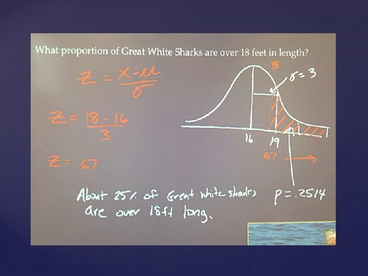
This is a sample, so we will use the x-bar for the mean and the “s” for the standard deviation. N(16, 3)

Sketch a Normal curve using the following as the mean and standard deviation for Great White Shark lengths. N(16, 3)

What proportion of Great White Sharks are over 18 feet in length? N(16, 3)

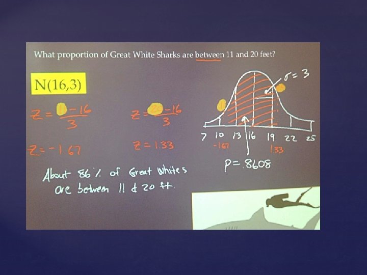
What proportion of Great White Sharks are between 11 and 20 feet? N(16, 3)

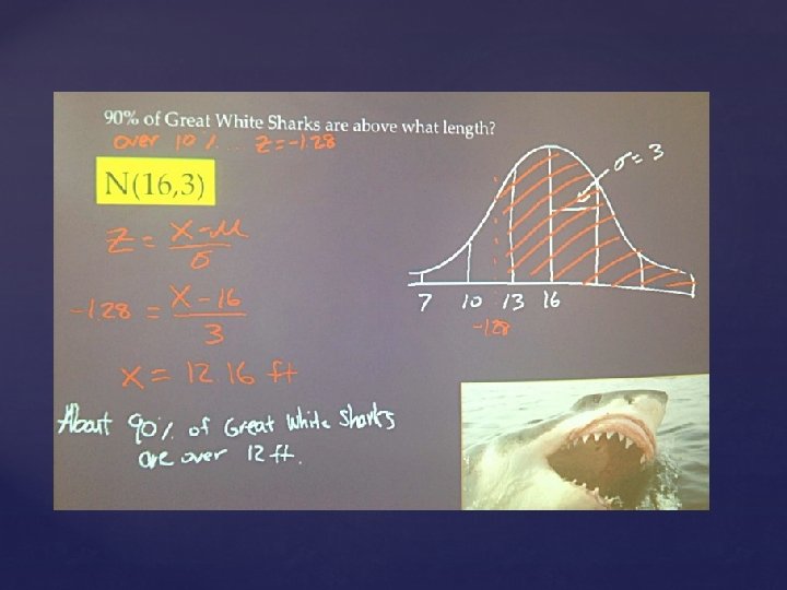
90% of Great White Sharks are above what length? N(16, 3)

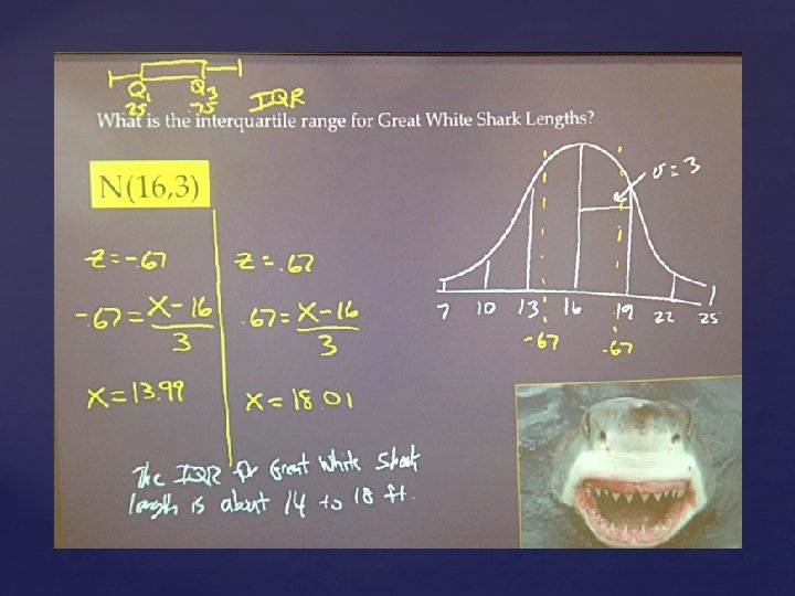
What is the interquartile range for Great White Shark Lengths? N(16, 3)

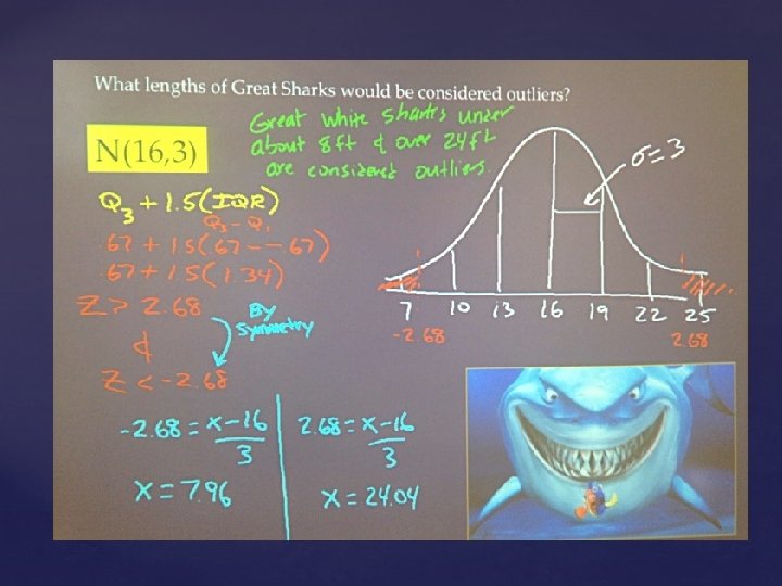
What lengths of Great Sharks would be considered outliers? N(16, 3)

COFFEE

The amount of coffee that Mr. Pines drinks on a school day follows a Normal Distribution with a mean of 23. 4 ounces and a standard deviation of 7. 2 ounces.

Mr. Pines coffee drinking N(23. 4, 7. 2) 1) Sketch a Normal curve labeling all important information for this situation 2) How often does Mr. Pines drink less than 20 ounces of coffee in a day? 3) How often does he drink between 15 and 30 ounces of coffee in a day? 4) 60% of the time he drinks more than ____ ounces of coffee in a day? 5) How many ounces of coffee would be considered outliers for Mr. Pines?

Mr. Pines coffee drinking N(23. 4, 7. 2) 1) Sketch a Normal curve labeling all important information for this situation

Mr. Pines coffee drinking N(23. 4, 7. 2) 2) How often does Mr. Pines drink less than 20 ounces of coffee in a day?

Mr. Pines coffee drinking N(23. 4, 7. 2) 3) How often does he drink between 15 and 30 ounces of coffee in a day?

Mr. Pines coffee drinking N(23. 4, 7. 2) 4) 60% of the time he drinks more than ____ ounces of coffee in a day?

Mr. Pines coffee drinking N(23. 4, 7. 2) 5) How many ounces of coffee would be considered outliers for Mr. Pines?

Tiger Woods

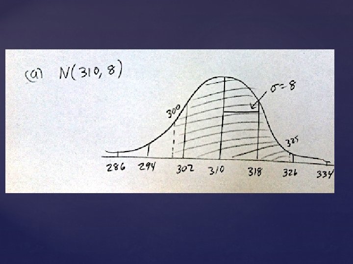
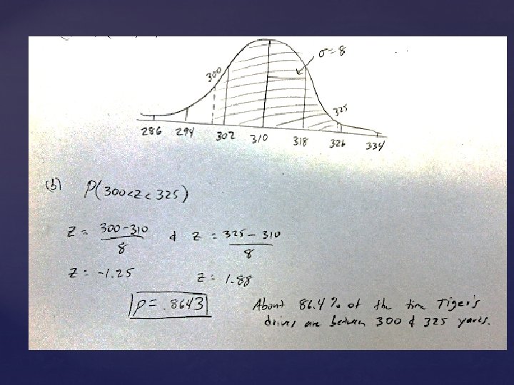
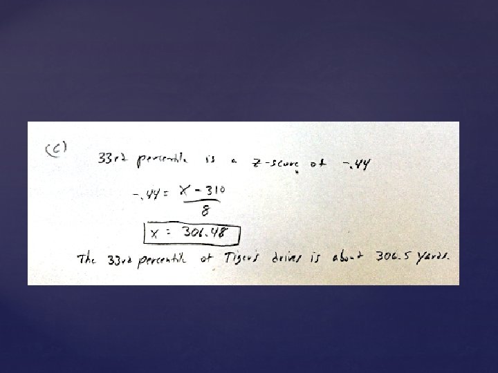
When Tiger Woods is on the driving range, the distance that golf balls travel when he hits them with a driver follows a Normal distribution with mean 310 yards and a standard deviation of 8 yards. a) Sketch the distribution of Tiger Wood’s drive distances. Label the points one, two, and three standard deviations from the mean. b) What proportion of Tiger’s drives travel between 300 and 325 yards? Shade the appropriate area under the curve you drew in (a). Then show your work. c) Find the 33 rd percentile of Tiger’s drive distance distribution. Show your method. d) What driving distances would be considered outliers for Tiger?

You need to remember the outlier formulas: Q 1 – 1. 5(IQR) Q 3 + 1. 5(IQR) Outliers on a Normal Curve

Q 1 is the 25 th percentile Q 3 is the 75 th percentile Why? Outliers on a Normal Curve

inv. Norm(. 25) = -. 67 inv. Norm(. 75) =. 67 IQR = Q 3 – Q 1 IQR =. 67 – (-. 67) = 1. 34 Q 1 – 1. 5(IQR) -. 67 – 1. 5(1. 34) = -2. 68 Q 3 + 1. 5(IQR) . 67 + 1. 5(1. 34) = 2. 68 Outliers on a Normal Curve

z = -2. 68 z = 2. 68 Outliers on a Normal Curve

z = -2. 68 z = -. 67 Q 1 z =. 67 Q 3 z = 2. 68 Outliers on a Normal Curve

IQR = 1. 34 Q 1 Q 3 Outliers on a Normal Curve

Brushing Teeth Mr. Pines typically brushes his teeth during break after he has finished his second cup of coffee. The amount of time he spends brushing his teeth follows a normal distribution with unknown mean and standard deviation. Mr. Pines spends less than one minute brushing his teeth about 40% of the time. He spends more than two minutes brushing his teeth 2% of the time. a) Use this information to determine the mean and standard deviation of this distribution. b) After you find the mean and standard deviation, sketch a normal curve labeling all the important information. (If your part “a” is correct then your normal curve will match the given percentages)

Brushing Teeth Use inv. Norm to get your Z-scores. inv. Norm(. 40) = -. 25 inv. Norm(. 98) = 2. 05 Set them equal to each other Plug the Stdev into any equation above to get a mean of 1. 11