The normal distribution Binomial distribution is discrete events

The normal distribution Binomial distribution is discrete events, (infected, not infected) The normal distribution is a probability density function for a continuous variable, and is represented by a continuous curve. Density = relative frequency of varites on the Y (horizontal) axis.

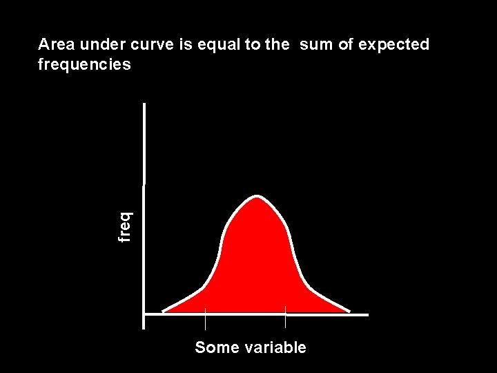
freq Area under curve is equal to the sum of expected frequencies Some variable

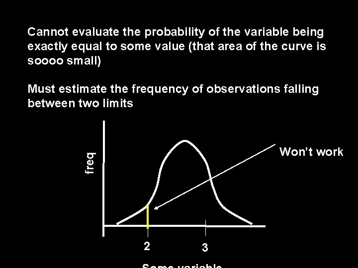
Cannot evaluate the probability of the variable being exactly equal to some value (that area of the curve is soooo small) Must estimate the frequency of observations falling between two limits freq Won’t work 2 3

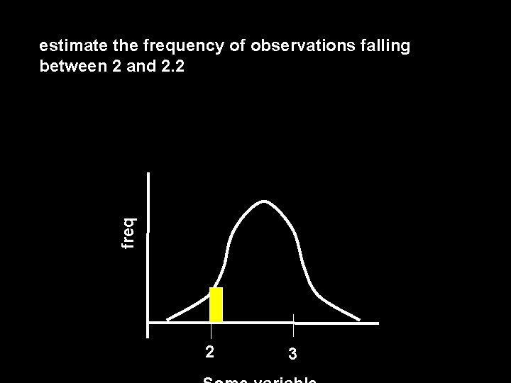
freq estimate the frequency of observations falling between 2 and 2. 2 2 3

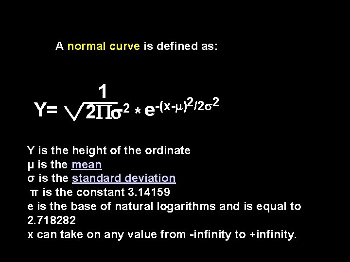
A normal curve is defined as: Y= 1 2/2 2 -(x- ) 2 2 * e Y is the height of the ordinate μ is the mean σ is the standard deviation π is the constant 3. 14159 e is the base of natural logarithms and is equal to 2. 718282 x can take on any value from -infinity to +infinity.

How is a normal probability distribution like a lion? They both have a MEAN MEW.

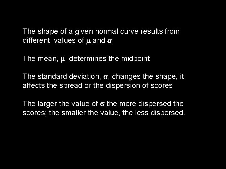
The shape of a given normal curve results from different values of and The mean, , determines the midpoint The standard deviation, , changes the shape, it affects the spread or the dispersion of scores The larger the value of the more dispersed the scores; the smaller the value, the less dispersed.

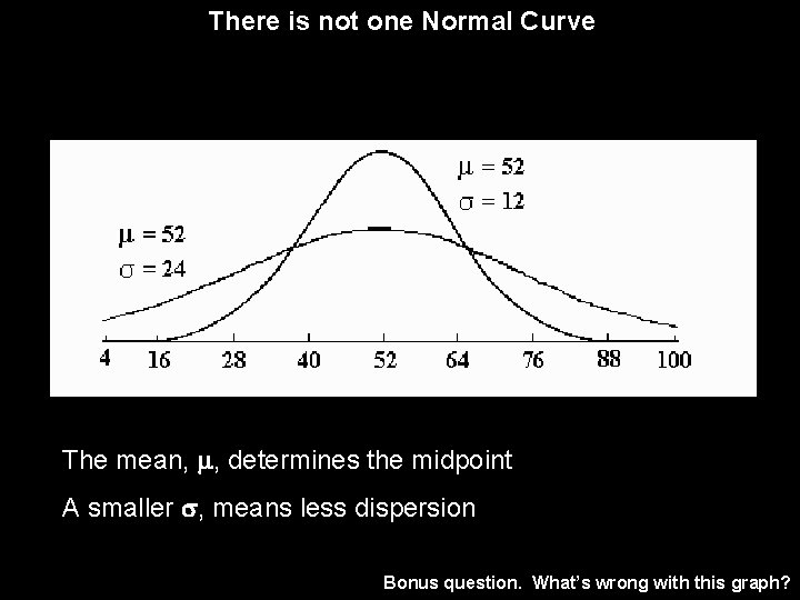
There is not one Normal Curve The mean, , determines the midpoint A smaller , means less dispersion Bonus question. What’s wrong with this graph?

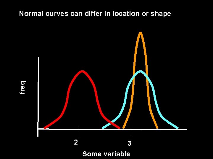
freq Normal curves can differ in location or shape 2 3 Some variable

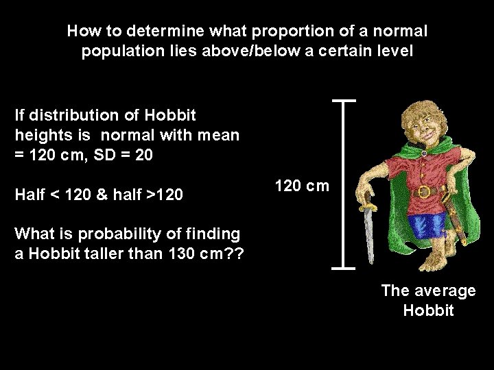
How to determine what proportion of a normal population lies above/below a certain level If distribution of Hobbit heights is normal with mean = 120 cm, SD = 20 Half < 120 & half >120 cm What is probability of finding a Hobbit taller than 130 cm? ? The average Hobbit

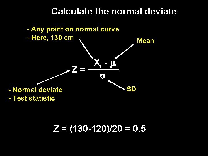
Calculate the normal deviate - Any point on normal curve - Here, 130 cm Mean Xi - Z= - Normal deviate - Test statistic SD Z = (130 -120)/20 = 0. 5

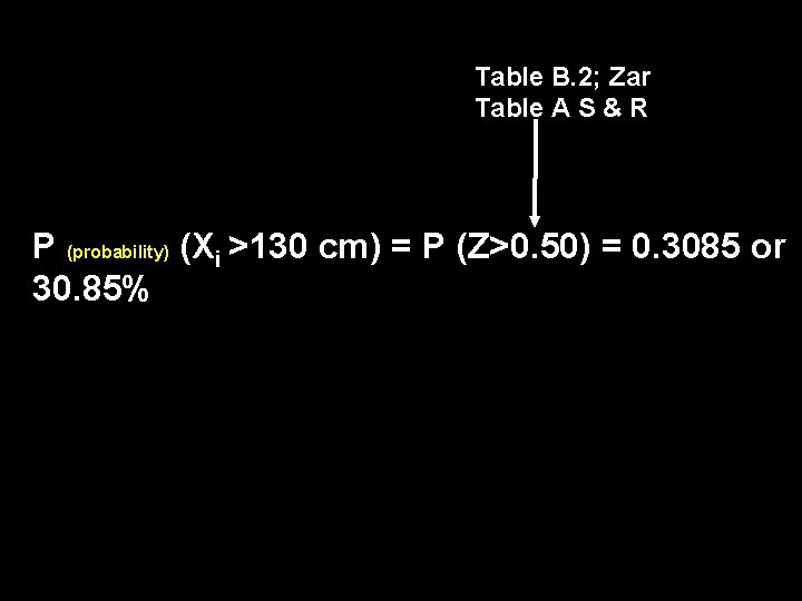
Table B. 2; Zar Table A S & R P (probability) (Xi >130 cm) = P (Z>0. 50) = 0. 3085 or 30. 85%

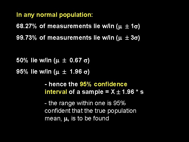
In any normal population: 68. 27% of measurements lie w/in ( 1 ) 99. 73% of measurements lie w/in ( 3 ) 50% lie w/in ( 0. 67 ) 95% lie w/in ( 1. 96 ) - hence the 95% confidence interval of a sample = X 1. 96 * s - the range within one is 95% confident that the true population mean, , is to be found

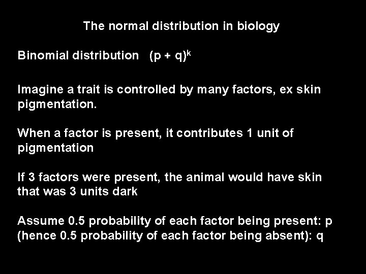
The normal distribution in biology Binomial distribution (p + q)k Imagine a trait is controlled by many factors, ex skin pigmentation. When a factor is present, it contributes 1 unit of pigmentation If 3 factors were present, the animal would have skin that was 3 units dark Assume 0. 5 probability of each factor being present: p (hence 0. 5 probability of each factor being absent): q

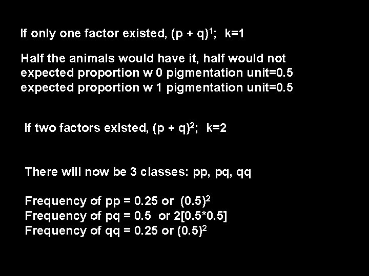
If only one factor existed, (p + q)1; k=1 Half the animals would have it, half would not expected proportion w 0 pigmentation unit=0. 5 expected proportion w 1 pigmentation unit=0. 5 If two factors existed, (p + q)2; k=2 There will now be 3 classes: pp, pq, qq Frequency of pp = 0. 25 or (0. 5)2 Frequency of pq = 0. 5 or 2[0. 5*0. 5] Frequency of qq = 0. 25 or (0. 5)2

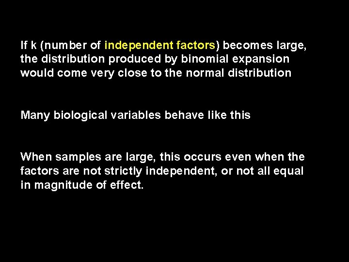
If k (number of independent factors) becomes large, the distribution produced by binomial expansion would come very close to the normal distribution Many biological variables behave like this When samples are large, this occurs even when the factors are not strictly independent, or not all equal in magnitude of effect.

Assessing Normality I'm not an outlier; I just haven't found my distribution yet

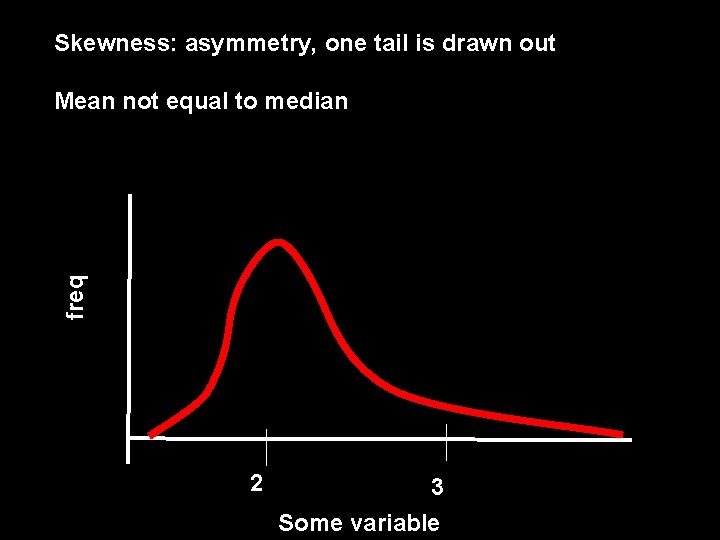
Skewness: asymmetry, one tail is drawn out freq Mean not equal to median 2 3 Some variable

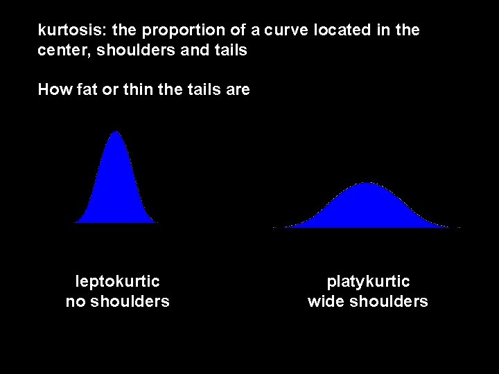
kurtosis: the proportion of a curve located in the center, shoulders and tails How fat or thin the tails are leptokurtic no shoulders platykurtic wide shoulders

More later on assessing normality using SAS

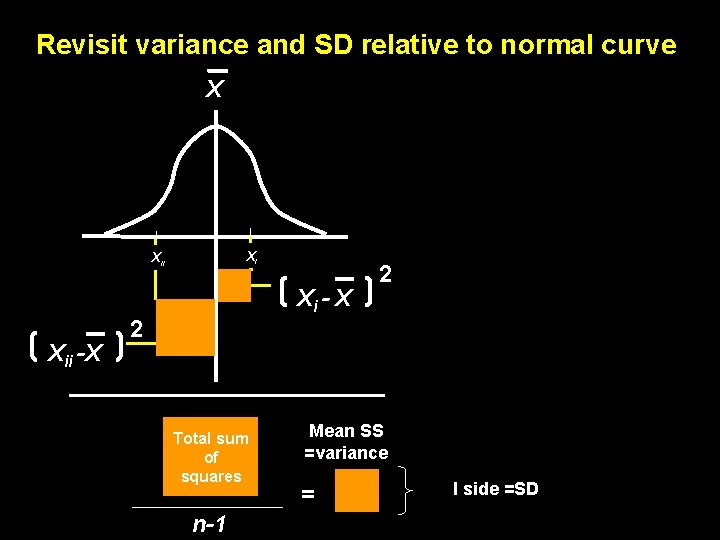
Revisit variance and SD relative to normal curve X Xi Xi - X Xii -X 2 2 Total sum of squares n-1 Mean SS =variance = I side =SD

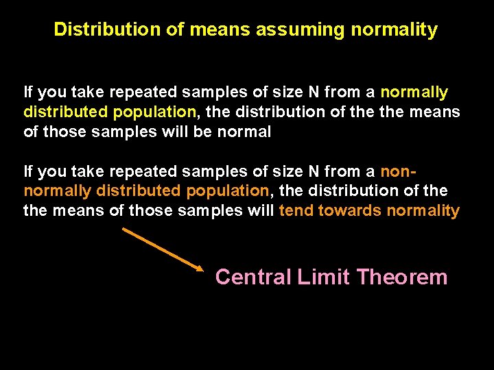
Distribution of means assuming normality If you take repeated samples of size N from a normally distributed population, the distribution of the means of those samples will be normal If you take repeated samples of size N from a nonnormally distributed population, the distribution of the means of those samples will tend towards normality Central Limit Theorem

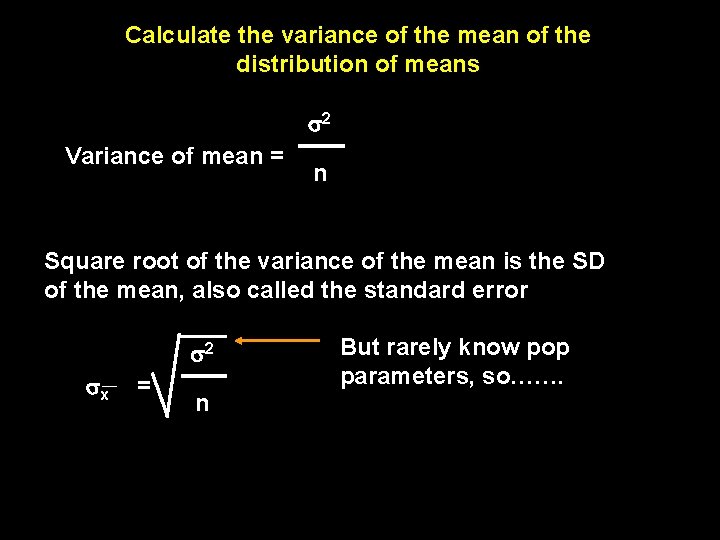
Calculate the variance of the mean of the distribution of means 2 Variance of mean = n Square root of the variance of the mean is the SD of the mean, also called the standard error 2 x = n But rarely know pop parameters, so…….

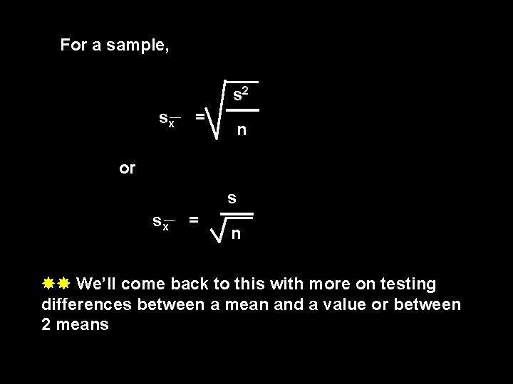
For a sample, s 2 sx = n or s sx = n We’ll come back to this with more on testing differences between a mean and a value or between 2 means

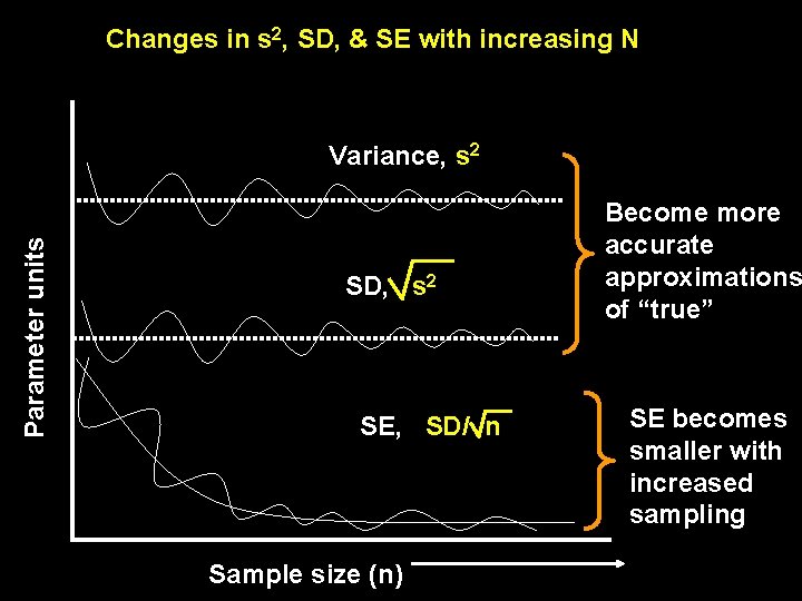
Changes in s 2, SD, & SE with increasing N Parameter units Variance, s 2 SD, s 2 SE, SD/ n Sample size (n) Become more accurate approximations of “true” SE becomes smaller with increased sampling

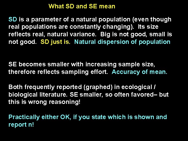
What SD and SE mean SD is a parameter of a natural population (even though real populations are constantly changing). Its size reflects real, natural variance. Big is not good, small is not good. SD just is. Natural dispersion of population SE becomes smaller with increasing sample size, therefore reflects sampling effort. Accuracy of mean. Both frequently reported (graphed) in ecological / biological literature. SE smaller, so often favored– but this is wrong reasoning! Practically either OK, if you state which is shown and report n!