The Memory Hierarchy Typically magnetic disks magneto optical

The Memory Hierarchy Typically magnetic disks, magneto optical (erasable), CD ROM. • Access times in milliseconds, great variability. • Unit of read/write = block or page, typically 16 Kb. • Capacities in gigabytes. Desired data carried to read/write port, access times in seconds. Most common: racks of tapes; newer devices: CD ROM “juke boxes, ” tape “silo's. ” Capacities in terabytes. under a microsecond, random access, perhaps 512 Mb fastest, but small

Volatile vs. Non Volatile A storage device is nonvolatile if it can retain its data after a power shutoff. Volatile

Computer Quantities Roughly: K M G T P Kilo Mega Giga Tera Peta

Disks • Platters with top and bottom surfaces rotate around a spindle. • Diameters 1 inch to 4 feet. • 2 --30 surfaces. • Rotation speed: 3600 --7200 rpm. • One head per surface. • All heads move in and out in unison.

Tracks and sectors • Surfaces are covered with concentric tracks. – Tracks at a common radius = cylinder. – Important because all data of a cylinder can be read quickly, without moving the heads. – Typical magnetic disk: 16, 000 cylinders • Tracks are divided into sectors by unmagnetized gaps (which are 10% of track). – Typical track: 512 sectors. – Typical sector: 4096 bytes. • Sectors are grouped into blocks. – Typical: one 16 K block = 4 4096 byte sectors.

MEGATRON 747 Disk Parameters • • • There are 8 platters providing 16 surfaces. There are 214, or 16, 384 tracks per surface. There are (on average) 27= 128 sectors per track. There are 212=4096=4 K bytes per sector. Capacity = 16*214*27*212 = 237 = 128*230 = 128 GB

Disk Controller 1. Buffer data in and out of disk. 2. Schedule the disk heads. 3. Manage the "bad blocks'' so they are not used.

Disk access time • Latency of the disk (access time): The time to bring block X, to main memory, from disk after the “read block” command is issued. • Main components of access time are: – Seek time = time to move heads to proper cylinder. – Rotational delay = time for desired block to come under head. – Transfer time = time during which the block passes under head. – Others, including CPU time to issue I/O, time for disk controller to process data, contention for the controller, bus, memory, etc. Negligible; “typical” value is 0!

Cause of rotational delay On average, the desired sector will be about half way around the circle when the heads arrive at the cylinder.

MEGATRON 747 Timing Example • Some timing properties of the Megatron 747 disk: – To move the head assembly between cylinders takes 1 ms to start and stop, plus 1 additional millisecond for every 1000 cylinders traveled. • Thus, moving from the innermost to the outermost track, a distance of 16, 383 tracks, is about 17. 38 milliseconds. – The disk rotates at 7200 rpm; i. e. , it makes one rotation in 8. 33 milliseconds. – To pass 16 K (4 sectors) under the head takes 0. 25 milliseconds. • Reading a block of 16 K takes in the worst case: 17. 38 + 8. 33 + 0. 25 = 25. 96 ms • Reading a block of 16 K takes in the best case: 0 + 0. 25 = 0. 25 ms • Reading a block of 16 K takes in average: Explanations about this are 17. 38/3 + 8. 33/2 + 0. 25 = 11 ms in the next slides.

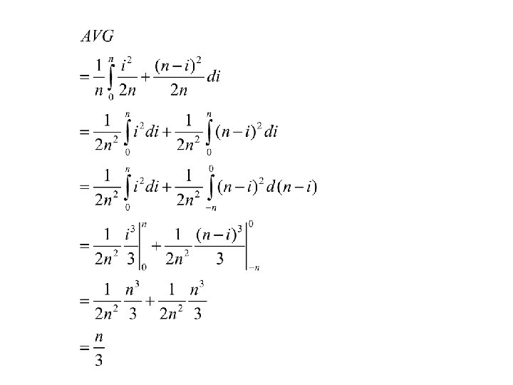
AVG time to read a 16, 384 byte block • Two of the components of the latency are easy to compute: – the transfer time is always 0. 25 milliseconds and – the average rotational latency is the time to rotate the disk half way around, or 4. 17 milliseconds. • We might suppose that the average seek time is just the time to move across half the tracks. Not quite right, since typically, the heads are initially somewhere near the middle and therefore will have to move less than half the distance, on average, to the desired cylinder. • • • Assume the heads are initially at any of the 16, 384 cylinders with equal probability. – If at cylinder 1 or cylinder 16, 384, then the average number of tracks to is about half i. e. 8192 tracks. – At the middle cylinder 8192, the head is equally likely to move in or out, and either way, it will move on average about a quarter of the tracks (4096) So, what’s the average number of tracks to travel?

AVG time to read a 16, 384 -byte block Average number of cyls to travel, if the heads are currently positioned at cyl i. Avg number of cyls to travel if the block is on the left. Probabilit y the block is on the left Avg number of cyls to travel if the block is on the right. Probabilit y the block is on the right

Writing and Modifying Blocks • Writing same as reading, unless we verify written blocks. • Modifying a block requires: 1. Read the block into main memory. 2. Modify the block there. 3. Write the block back to disk.

Using Secondary Storage Effectively • In most studies of algorithms, one assumes the “RAM model”: – Data is in main memory, – Access to any item of data takes as much time as any other. • When implementing a DBMS, one must assume that the data does not fit into main memory. • Often, the best algorithms for processing very large amounts of data differ from the best main memory algorithms for the same problem. – There is a great advantage in choosing an algorithm that uses few disk accesses, even if the algorithm is not very efficient when viewed as a main memory algorithm.

Assumptions • One processor • One disk controller, and one disk. • The database itself is much too large to fit in main memory. • Many users, and each user issues disk I/O requests frequently, – Disk controller serving on a first come first served basis. – Requests for a given user might appear random even if the table that a user is reading is stored on a single cylinder of the disk. • The disk is a Megatron 747, with 16 K blocks and the timing characteristics determined before. • In particular, the average time to read or write a block is about 11 ms

I/O model of computation • Disk I/O = read or write of a block is very expensive compared with what is likely to be done with the block once it arrives in main memory. – Perhaps 1, 000 machine instructions in the time to do one random disk I/O. Good DBMS algorithms • Try to make sure that if we read a block, we use much of the data on the block.

Merge Sort • Common main memory sorting algorithms don't look so good when you take disk I/O's into account. Variants of Merge Sort do better. • Merge = take two sorted lists and repeatedly chose the smaller of the “heads” of the lists (head = first of the unchosen). – Example: merge 1, 3, 4, 8 with 2, 5, 7, 9 = 1, 2, 3, 4, 5, 7, 8, 9. • Merge Sort based on recursive algorithm: divide records into two parts; recursively mergesort the parts, and merge the resulting lists.

Two Phase, Multiway Merge Sort still not very good in disk I/O model. • log 2 n passes, so each record is read/written from disk log 2 n times. • The secondary memory algorithms operate in a small number of passes; – in one pass every record is read into main memory once and written out to disk once. • 2 PMMS: 2 reads + 2 writes per block. • Phase 1 1. Fill main memory with records. 2. Sort using favorite main memory sort. 3. Write sorted sublist to disk. 4. Repeat until all records have been put into one of the sorted lists.

Phase 2 • Use one buffer for each of the sorted sublists and one buffer for an output block. • Initially load input buffers with the first blocks of their respective sorted lists. • Repeatedly run a competition among the first unchosen records of each of the buffered blocks. • Move the record with the least key to the output block; it is now “chosen. ” • Manage the buffers as needed: • If an input block is exhausted, get the next block from the same file. • If the output block is full, write it to disk.

Toy Example • 24 tuples with keys: – 12 10 25 20 40 30 27 29 14 18 45 23 70 65 35 11 49 47 22 21 46 34 29 39 • Suppose 1 block can hold 2 tuples. • Suppose main memory (MM) can hold 4 blocks i. e. 8 tuples. Phase 1. • Load 12 10 25 20 40 30 27 29 in MM, sort them and write the sorted sublist: 10 12 20 25 27 29 30 40 • Load 14 18 45 23 70 65 35 11 in MM, sort them and write the sorted sublist: 11 14 18 23 35 45 65 70 • Load 49 47 22 21 46 34 29 39 in MM, sort them and write the sorted sublist: 21 22 29 34 39 46 47 49

Toy example (continued) Phase 2. Sublist 1: 10 12 20 25 27 29 30 40 Sublist 2: 11 14 18 23 35 45 65 70 Sublist 3: 21 22 29 34 39 46 47 49 Main Memory (4 buffers) Input Buffer 1: Input Buffer 2: Input Buffer 3: Output Buffer: Sorted list:

Toy example (continued) Phase 2. Sublist 1: 20 25 27 29 30 40 Sublist 2: 18 23 35 45 65 70 Sublist 3: 29 34 39 46 47 49 Main Memory (4 buffers) Input Buffer 1: 10 12 Input Buffer 2: 11 14 Input Buffer 3: 21 22 Output Buffer: Sorted list:

Toy example (continued) Phase 2. Sublist 1: 20 25 27 29 30 40 Sublist 2: 18 23 35 45 65 70 Sublist 3: 29 34 39 46 47 49 Main Memory (4 buffers) Input Buffer 1: 12 Input Buffer 2: 11 14 Input Buffer 3: 21 22 Output Buffer: 10 Sorted list:

Toy example (continued) Phase 2. Sublist 1: 20 25 27 29 30 40 Sublist 2: 18 23 35 45 65 70 Sublist 3: 29 34 39 46 47 49 Main Memory (4 buffers) Input Buffer 1: 12 Input Buffer 2: 14 Input Buffer 3: 21 22 Output Buffer: 10 11 Sorted list:

Toy example (continued) Phase 2. Sublist 1: 20 25 27 29 30 40 Sublist 2: 18 23 35 45 65 70 Sublist 3: 29 34 39 46 47 49 Main Memory (4 buffers) Input Buffer 1: 12 Input Buffer 2: 14 Input Buffer 3: 21 22 Output Buffer: Sorted list: 10 11

Toy example (continued) Phase 2. Sublist 1: 20 25 27 29 30 40 Sublist 2: 18 23 35 45 65 70 Sublist 3: 29 34 39 46 47 49 Main Memory (4 buffers) Input Buffer 1: Input Buffer 2: 14 Input Buffer 3: 21 22 Output Buffer: 12 Sorted list: 10 11

Toy example (continued) Phase 2. Sublist 1: 27 29 30 40 Sublist 2: 18 23 35 45 65 70 Sublist 3: 29 34 39 46 47 49 Main Memory (4 buffers) Input Buffer 1: 20 25 Input Buffer 2: 14 Input Buffer 3: 21 22 Output Buffer: 12 Sorted list: 10 11

Toy example (continued) Phase 2. Sublist 1: 27 29 30 40 Sublist 2: 18 23 35 45 65 70 Sublist 3: 29 34 39 46 47 49 Main Memory (4 buffers) Input Buffer 1: 20 25 Input Buffer 2: Input Buffer 3: 21 22 Output Buffer: 12 14 Sorted list: 10 11

Toy example (continued) Phase 2. Sublist 1: 27 29 30 40 Sublist 2: 18 23 35 45 65 70 Sublist 3: 29 34 39 46 47 49 Main Memory (4 buffers) Input Buffer 1: 20 25 Input Buffer 2: Input Buffer 3: 21 22 Output Buffer: Sorted list: 10 11 12 14

Toy example (continued) Phase 2. Sublist 1: 27 29 30 40 Sublist 2: 35 45 65 70 Sublist 3: 29 34 39 46 47 49 Main Memory (4 buffers) Input Buffer 1: 20 25 Input Buffer 2: 18 23 Input Buffer 3: 21 22 Output Buffer: Sorted list: 10 11 12 14 We continue in this way until the sorted sublists are finished and we get the whole sorted list of tuples.

Real Life Example • 10, 000 tuples of 160 bytes = 1. 6 Gb file. – Stored on Megatron 747 disk, with 16 K blocks, each holding 100 tuples – Entire file takes 100, 000 blocks • 100 M bytes available main memory – The number of blocks that can fit in 100 M bytes of memory (which, recall, is really 100 x 220 bytes), is 100 x 220/214, or 6400 blocks 1/16 th of file. • Sort by primary key field.

Analysis – Phase 1 • 6400 of the 100, 000 blocks will fill main memory. • We thus fill memory 100, 000/6, 400 =16 times, sort the records in main memory, and write the sorted sublists out to disk. • How long does this phase take? • We read each of the 100, 000 blocks once, and we write 100, 000 new blocks. Thus, there are 200, 000 disk I/O's for 200, 000*11 ms = 2200 seconds, or 37 minutes. Avg. time for reading a block.

Analysis – Phase 2 • Every block holding records from one of the sorted lists is read from disk exactly once. – Thus, the total number of block reads is 100, 000 in the second phase, just as for the first. • Likewise, each record is placed once in an output block, and each of these blocks is written to disk. – Thus, the number of block writes in the second phase is also 100, 000. • We conclude that the second phase takes another 37 minutes. • Total: Phase 1 + Phase 2 = 74 minutes.

How Big Should Blocks Be? • We have assumed a 16 K byte block in our analysis. • However, there arguments that a larger block size would be advantageous. • If we doubled the size of blocks, we would halve the number of disk I/O's. • But, how much a disk I/O would cost in such a case? • Recall it takes about – 0. 25 ms for transfer time of a 16 K block and – 10. 63 milliseconds for average seek time and rotational latency. • Now, the only change in the time to access a block would be that the transfer time increases to 0. 25*2=0. 50 millisecond, i. e. only slightly more than before. – We would thus approximately halve the time the sort takes.

Another example: Block Size = 512 K • For a block size of 512 K (i. e. , an entire track of the Megatron 747) the transfer time is 0. 25*32=8 milliseconds. • Average block access time would be 10. 63 + 8 approx. 19 ms, (as opposed to 11 ms we had) • However, now a block can hold 100*32 = 3200 tuples and the whole table will be 10, 000 / 3200 = 3125 blocks (as opposed to 100, 000 blocks we had before). • Thus, we would need only 3125 * 2 disk I/Os for 2 PMMS for a total time of 3125 * 2 * 19 = 237, 500 ms or about 4 min. • Speedup: 74 / 4 = 18 fold.

Reasons to limit the block size 1. First, we cannot use blocks that cover several tracks effectively. 2. Second, small relations would occupy only a fraction of a block, so large blocks would waste space on the disk. 3. Third, the larger the blocks are, the fewer records we can sort by 2 PMMS (see next slide). • Nevertheless, as machines get more memory and disks more capacious, there is a tendency for block sizes to grow.

How many records can we sort? 1. 2. 3. Block size is B bytes. Main memory available for buffering blocks is M bytes. Records take R bytes. • • Number of main memory buffers = M/B blocks We need one output buffer, so we can actually use (M/B) 1 input buffers. • • How many sorted sublists makes sense to produce? (M/B) 1. • • • What’s the total number of records we can sort? Each time we fill in the memory with M/R records. Hence, we are able to sort (M/R)*[(M/B) 1] or approximately M 2/RB. If we use the parameters in the example about TPMMS we have: M=100 MB = 100, 000 Bytes = 108 Bytes B = 16, 384 Bytes R = 160 Bytes So, M 2/RB = (108)2 / (160 * 16, 384) = 4. 2 billion records, or 2/3 of a Tera. Byte.

Sorting larger relations • If our relation is bigger, then, we can use 2 PMMS to create sorted sublists of M 2/RB records. • Then, in a third pass we can merge (M/B)-1 of these sorted sublists. • Thus, the third phase let’s us sort • [(M/B)-1]*[M 2/RB] M 3/RB 2 records • For our example, the third phase let’s us sort 75 trillion records occupying 7500 Petabytes!!