The MAP 3 S StaticandRegular Mesh Simulation and

Pattern-based parallel-programming • Observation: – Many seemingly different parallel programs have a common parallel

MAP 3 S • MAP 3 S = MPI/C Advanced Pattern-based Parallel Programming System

Pattern-based parallel-programming • The MAP 3 S usage scheme: Select Pattern Create Specification File

The Simulation and Wavefront computations • The computations operate on a k-dimensional mesh of

Mesh-blocks • A k-dimensional mesh is logically partitioned into kdimensional sub-meshes called mesh-blocks. 0

User-side code: Simulation Prelude: process command-line arguments. Prelude Prologue Body. Local Body. Global: decide

User-side code: Wavefront Prelude: process command-line arguments Prologue: initialize mesh, possibly at granularity of

Data-dependency specification • The computation of an element depends on the values of certain

Data-dependency specification • The strengths of conditional shape-lists: • user is not limited to

Direct mesh-access • In the user-code all the mesh elements can be accessed directly.

Engine-side code in the Wavefront pattern. 0 1 2 3 4 5 6 7

Engine-side code • The mesh-block-level data-dependencies are utilized to establish a parallel-computation schedule. 0

Engine-side code CPU 0 • The parallel computation-schedule is refined with mesh-blocks being assigned

Engine-side code CPU 0 • Execution of user-side code by the engine-side code when

Mesh representation • The mesh can be represented using either the dense mesh-representation or

Mesh representation • A mesh memory-footprint can be as much a problem as performance.

Experimental evaluation • Problems: – 2 D problems: • Go. L: game-of-life (Simulation) •

Experimental evaluation • Speedup on Gig. E: – x-axis is # of nodes. –

Experimental evaluation • Speedup on IB: – x-axis is # of nodes. – y-axis

Experimental evaluation • Capability: – Use of sparse-mesh representation distributes the mesh memoryfootprint across

Experimental evaluation • What we learned: – Dense meshes + large computation granularity: •

Slides: 29

Download presentation

The MAP 3 S Static-and-Regular Mesh Simulation and Wavefront Parallel-Programming Patterns By Robert Niewiadomski, José Nelson Amaral, and Duane Szafron Department of Computing Science University of Alberta Edmonton, Alberta, Canada

Pattern-based parallel-programming • Observation: – Many seemingly different parallel programs have a common parallel computation-communication-synchronization pattern. • A Parallel-programming pattern instance: – Is a parallel program that adheres to a certain parallel computationcommunication-synchronization pattern. – Consists of engine-side code and user-side code: • Engine-side code: – Is complete and handles all communication and synchronization. • User-side code: – Is incomplete and handles all computation. – User completes the incomplete portions. • MAP 3 S targets distributed-memory systems.

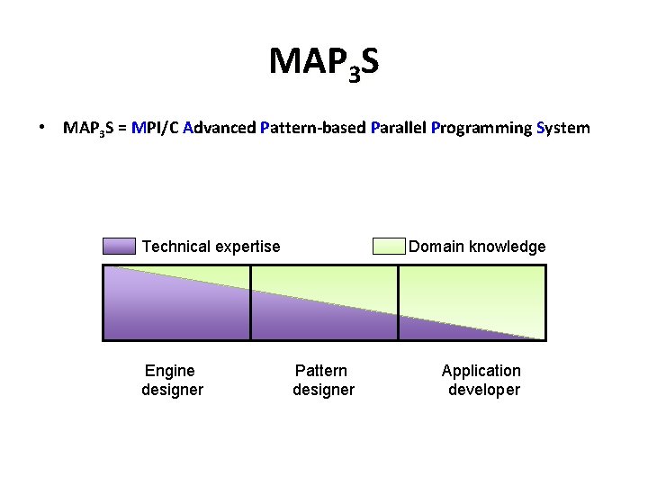
MAP 3 S • MAP 3 S = MPI/C Advanced Pattern-based Parallel Programming System Technical expertise Engine designer Domain knowledge Pattern designer Application developer

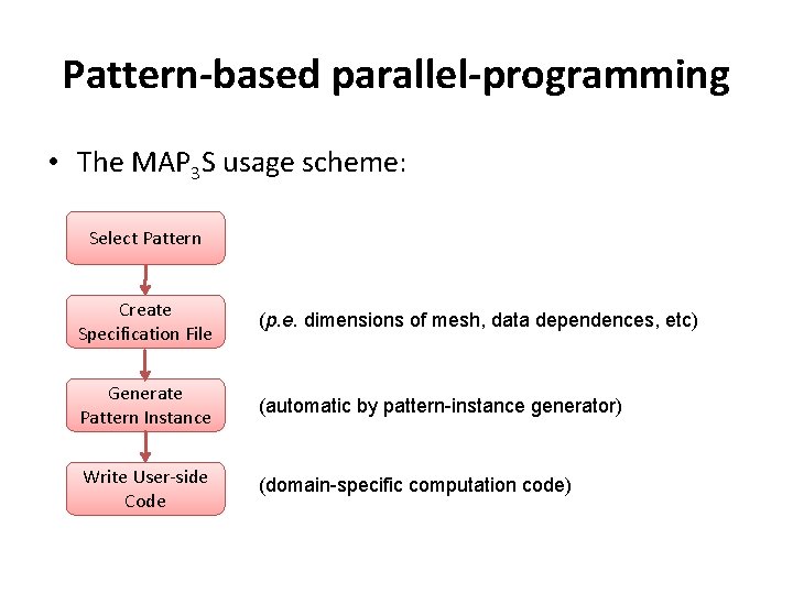
Pattern-based parallel-programming • The MAP 3 S usage scheme: Select Pattern Create Specification File (p. e. dimensions of mesh, data dependences, etc) Generate Pattern Instance (automatic by pattern-instance generator) Write User-side Code (domain-specific computation code)

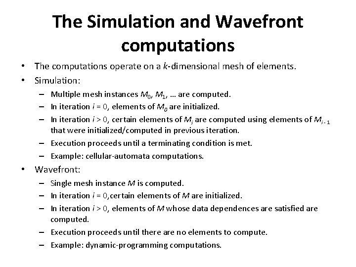
The Simulation and Wavefront computations • The computations operate on a k-dimensional mesh of elements. • Simulation: – Multiple mesh instances M 0, M 1, … are computed. – In iteration i = 0, elements of M 0 are initialized. – In iteration i > 0, certain elements of Mi are computed using elements of Mi - 1 that were initialized/computed in previous iteration. – Execution proceeds until a terminating condition is met. – Example: cellular-automata computations. • Wavefront: – Single mesh instance M is computed. – In iteration i = 0, certain elements of M are initialized. – In iteration i > 0, elements of M whose data dependences are satisfied are computed. – Execution proceeds until there are no elements to compute. – Example: dynamic-programming computations.

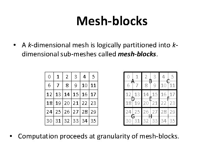
Mesh-blocks • A k-dimensional mesh is logically partitioned into kdimensional sub-meshes called mesh-blocks. 0 1 2 3 4 5 0 6 7 8 9 10 11 6 A 1 2 7 8 B 3 4 C 5 9 10 11 12 13 14 15 16 17 18 19 20 21 22 23 24 25 26 27 28 29 30 31 32 33 34 35 D G E H F I • Computation proceeds at granularity of mesh-blocks.

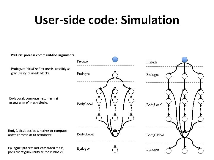
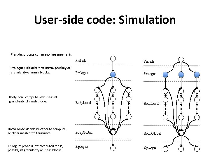
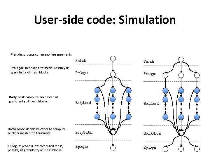
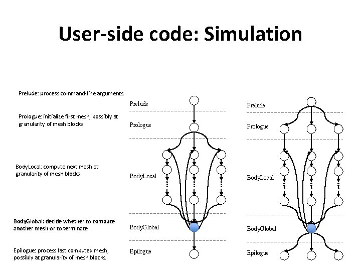
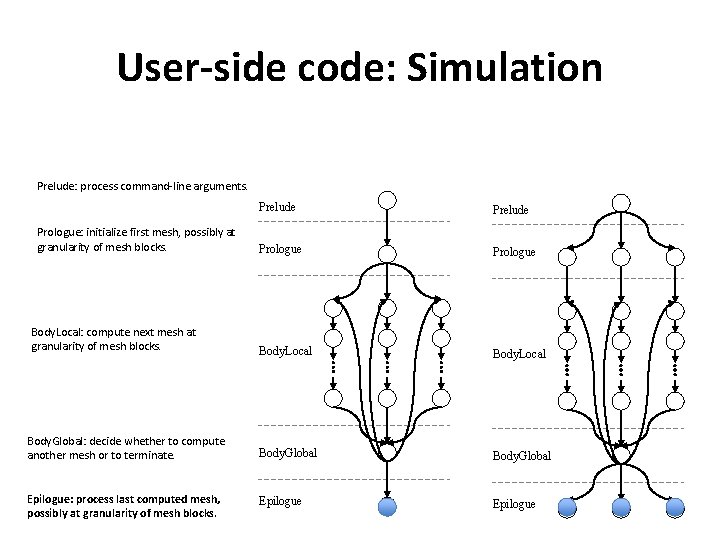
User-side code: Simulation Prelude: process command-line arguments. Prelude Prologue Body. Local Body. Global: decide whether to compute another mesh or to terminate. Body. Global Epilogue: process last computed mesh, possibly at granularity of mesh blocks. Epilogue Prologue: initialize first mesh, possibly at granularity of mesh blocks. Body. Local: compute next mesh at granularity of mesh blocks.

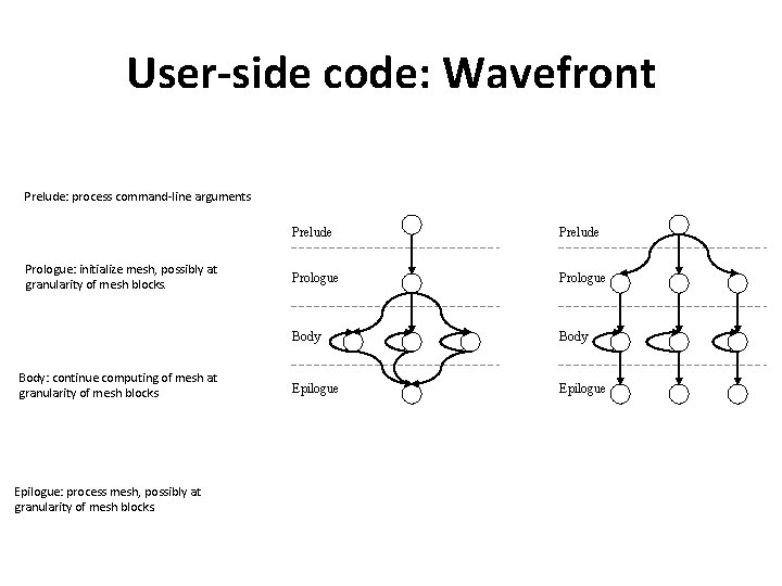
User-side code: Wavefront Prelude: process command-line arguments Prologue: initialize mesh, possibly at granularity of mesh blocks. Body: continue computing of mesh at granularity of mesh blocks Epilogue: process mesh, possibly at granularity of mesh blocks. Prelude Prologue Body Epilogue

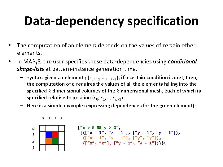
Data-dependency specification • The computation of an element depends on the values of certain other elements. • In MAP 3 S, the user specifies these data-dependencies using conditional shape-lists at pattern-instance generation time. – Syntax: given an element p(c 0, c 1, …, ck - 1), if a certain condition is met, then, the computation of p requires the values of all the elements falling into the specified k-dimensional volumes of the k-dimensional mesh, each of which is specified relative to position (c 0, c 1, …, ck - 1). – Here is a simple example (expressing dependences for the green element): 0 1 2 3 {“x > 0 && y > 0”, {([“x - 1”, ”x - 1”], [“y - 1”, “y - 1”]), ([“x - 1”, “x - 1”], [“y”, “y”]), ([“x”, “x”], [“y - 1”, ”y - 1”])}};

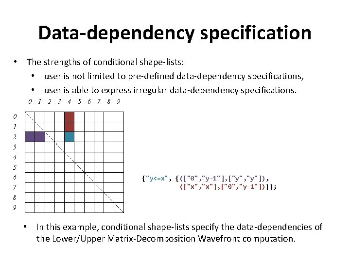
Data-dependency specification • The strengths of conditional shape-lists: • user is not limited to pre-defined data-dependency specifications, • user is able to express irregular data-dependency specifications. 0 1 2 3 4 5 6 7 8 9 {"y<=x", {(["0", "y-1"], ["y", "y"]), (["x", "x"], ["0", "y-1"])}}; • In this example, conditional shape-lists specify the data-dependencies of the Lower/Upper Matrix-Decomposition Wavefront computation.

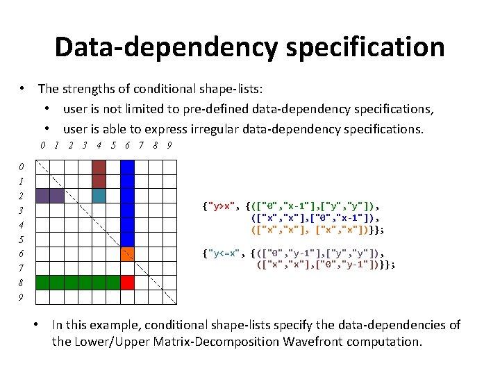
Data-dependency specification • The strengths of conditional shape-lists: • user is not limited to pre-defined data-dependency specifications, • user is able to express irregular data-dependency specifications. 0 1 2 3 4 5 6 7 8 9 {"y>x", {(["0", "x-1"], ["y", "y"]), (["x", "x"], ["0", "x-1"]), (["x", "x"], ["x", "x"])}}; {"y<=x", {(["0", "y-1"], ["y", "y"]), (["x", "x"], ["0", "y-1"])}}; • In this example, conditional shape-lists specify the data-dependencies of the Lower/Upper Matrix-Decomposition Wavefront computation.

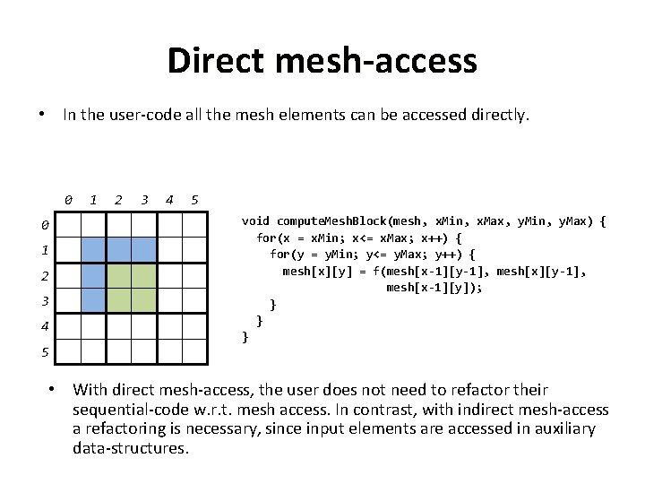
Direct mesh-access • In the user-code all the mesh elements can be accessed directly. 0 0 1 2 3 4 5 void compute. Mesh. Block(mesh, x. Min, x. Max, y. Min, y. Max) { for(x = x. Min; x<= x. Max; x++) { for(y = y. Min; y<= y. Max; y++) { mesh[x][y] = f(mesh[x-1][y-1], mesh[x-1][y]); } } } • With direct mesh-access, the user does not need to refactor their sequential-code w. r. t. mesh access. In contrast, with indirect mesh-access a refactoring is necessary, since input elements are accessed in auxiliary data-structures.

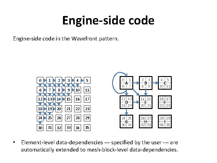
Engine-side code in the Wavefront pattern. 0 1 2 3 4 5 6 7 8 9 10 11 12 13 14 15 16 17 18 19 20 21 22 23 24 25 26 27 28 29 30 31 32 33 34 35 0 3 4 9 10 11 12 13 14 15 16 17 18 19 20 21 22 23 24 25 26 27 28 29 30 31 32 33 34 35 6 A 1 2 7 8 D G B E H C 5 F I • Element-level data-dependencies --- specified by the user --- are automatically extended to mesh-block-level data-dependencies.

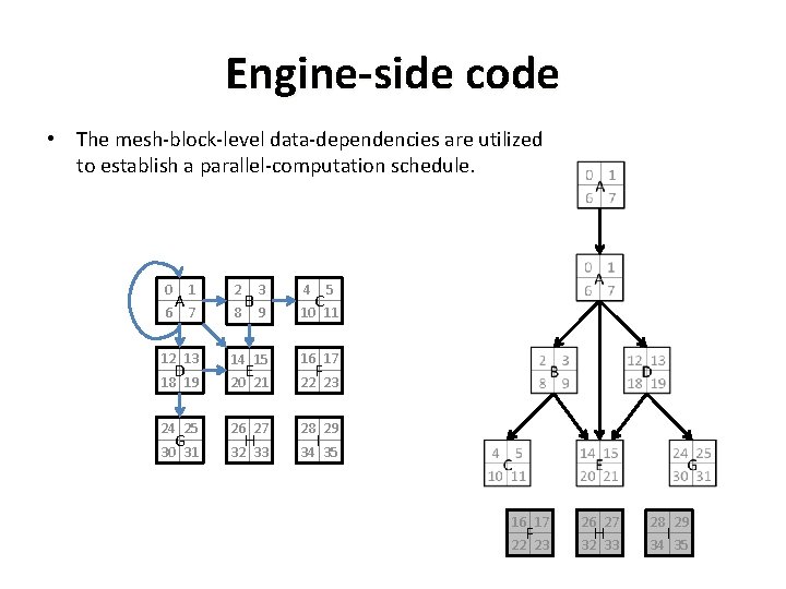
Engine-side code • The mesh-block-level data-dependencies are utilized to establish a parallel-computation schedule. 0 3 4 9 10 11 12 13 14 15 16 17 18 19 20 21 22 23 24 25 26 27 28 29 30 31 32 33 34 35 6 A 1 2 7 8 D G B E H C 5 F I 16 17 26 27 28 29 22 23 32 33 34 35 F H I

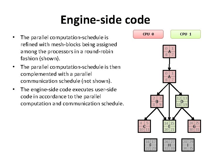
Engine-side code CPU 0 • The parallel computation-schedule is refined with mesh-blocks being assigned among the processors in a round-robin fashion (shown). • The parallel computation-schedule is then complemented with a parallel communication schedule (not shown). • The engine-side code executes user-side code in accordance to the parallel computation and communication schedule. CPU 1 0 6 2 8 4 B A A 1 7 3 12 13 9 18 19 D 5 14 15 24 25 10 11 20 21 30 31 C G E 16 17 26 27 28 29 22 23 32 33 34 35 F H I

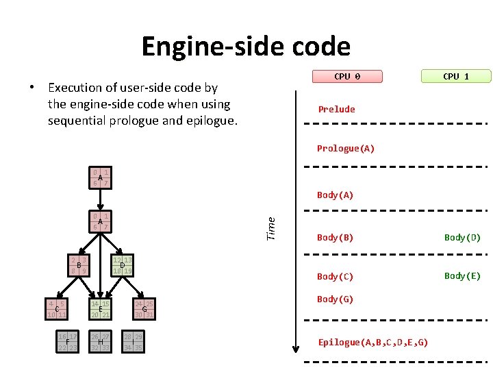
Engine-side code CPU 0 • Execution of user-side code by the engine-side code when using sequential prologue and epilogue. CPU 1 Prelude Prologue(A) 0 1 A 6 7 Body(A) 2 3 B 8 9 4 5 C 10 11 16 17 F 22 23 Time 0 1 A 6 7 12 13 D 18 19 14 15 E 20 21 26 27 H 32 33 24 25 G 30 31 28 29 I 34 35 Body(B) Body(D) Body(C) Body(E) Body(G) Epilogue(A, B, C, D, E, G)

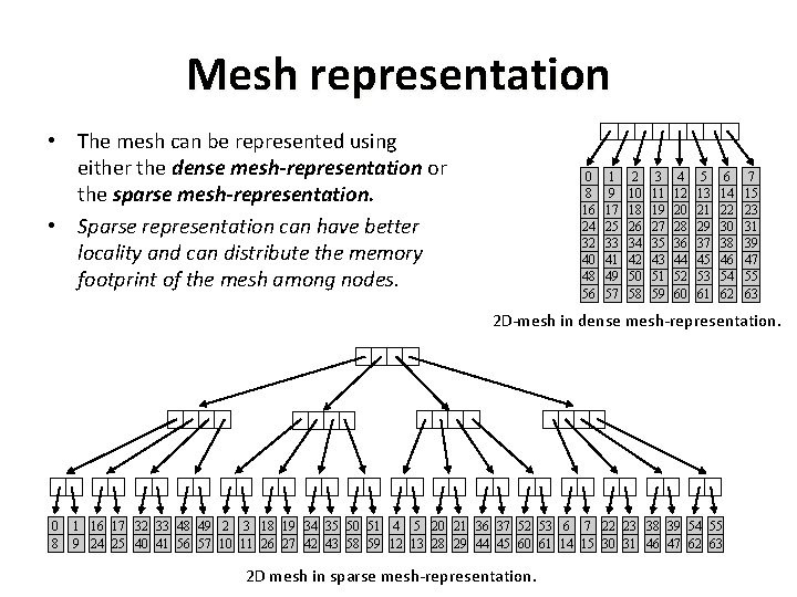
Mesh representation • The mesh can be represented using either the dense mesh-representation or the sparse mesh-representation. • Sparse representation can have better locality and can distribute the memory footprint of the mesh among nodes. 0 8 16 24 32 40 48 56 1 9 17 25 33 41 49 57 2 10 18 26 34 42 50 58 3 11 19 27 35 43 51 59 4 12 20 28 36 44 52 60 5 13 21 29 37 45 53 61 6 14 22 30 38 46 54 62 7 15 23 31 39 47 55 63 2 D-mesh in dense mesh-representation. 0 8 1 16 17 32 33 48 49 2 3 18 19 34 35 50 51 4 5 20 21 36 37 52 53 6 7 22 23 38 39 54 55 9 24 25 40 41 56 57 10 11 26 27 42 43 58 59 12 13 28 29 44 45 60 61 14 15 30 31 46 47 62 63 2 D mesh in sparse mesh-representation.

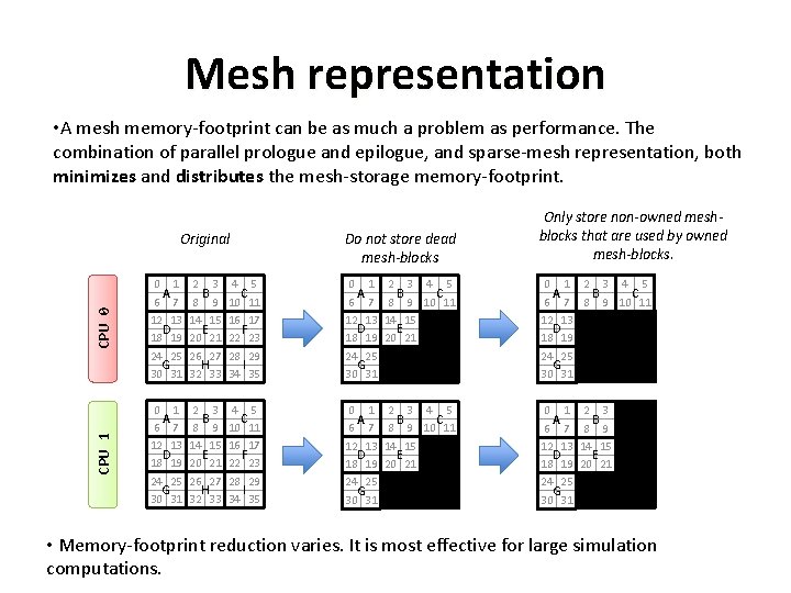
Mesh representation • A mesh memory-footprint can be as much a problem as performance. The combination of parallel prologue and epilogue, and sparse-mesh representation, both minimizes and distributes the mesh-storage memory-footprint. CPU 0 Do not store dead mesh-blocks 0 1 A 6 7 12 13 D 18 19 24 25 G 30 31 2 3 B 8 9 14 15 E 20 21 26 27 H 32 33 4 5 C 10 11 16 17 F 22 23 28 29 I 34 35 0 1 A 6 7 12 13 D 18 19 24 25 G 30 31 2 3 4 5 B C 8 9 10 11 14 15 E 20 21 0 1 2 3 4 5 A B C 6 7 8 9 10 11 12 13 D 18 19 24 25 G 30 31 CPU 1 Original Only store non-owned meshblocks that are used by owned mesh-blocks. 0 1 A 6 7 12 13 D 18 19 24 25 G 30 31 2 3 B 8 9 14 15 E 20 21 26 27 H 32 33 4 5 C 10 11 16 17 F 22 23 28 29 I 34 35 0 1 A 6 7 12 13 D 18 19 24 25 G 30 31 2 3 4 5 B C 8 9 10 11 14 15 E 20 21 0 1 A 6 7 12 13 D 18 19 24 25 G 30 31 2 3 B 8 9 14 15 E 20 21 • Memory-footprint reduction varies. It is most effective for large simulation computations.

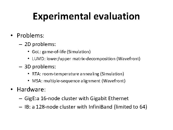
Experimental evaluation • Problems: – 2 D problems: • Go. L: game-of-life (Simulation) • LUMD: lower/upper matrix-decomposition (Wavefront) – 3 D problems: • RTA: room-temperature annealing (Simulation) • MSA: multiple-sequence alignment (Wavefront) • Hardware: – Gig. E: a 16 -node cluster with Gigabit Ethernet – IB: a 128 -node cluster with Infini. Band (limited to 64)

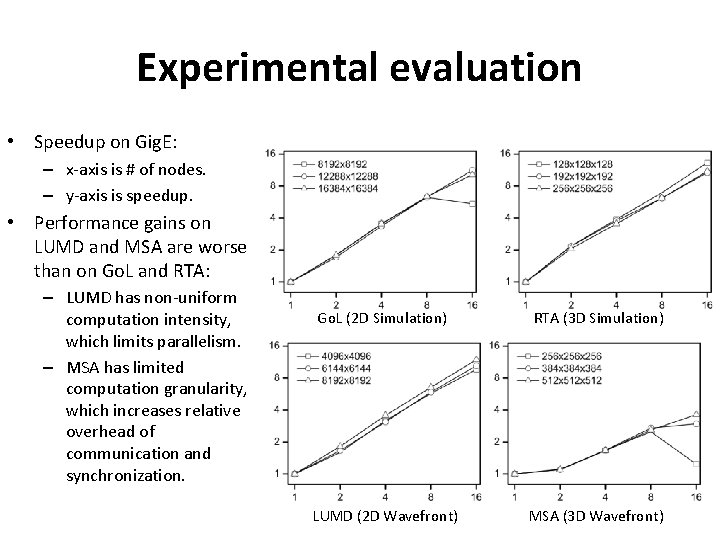
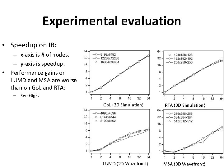
Experimental evaluation • Speedup on Gig. E: – x-axis is # of nodes. – y-axis is speedup. • Performance gains on LUMD and MSA are worse than on Go. L and RTA: – LUMD has non-uniform computation intensity, which limits parallelism. – MSA has limited computation granularity, which increases relative overhead of communication and synchronization. Go. L (2 D Simulation) RTA (3 D Simulation) LUMD (2 D Wavefront) MSA (3 D Wavefront)

Experimental evaluation • Speedup on IB: – x-axis is # of nodes. – y-axis is speedup. • Performance gains on LUMD and MSA are worse than on Go. L and RTA: – See Gig. E. Go. L (2 D Simulation) LUMD (2 D Wavefront) RTA (3 D Simulation) MSA (3 D Wavefront)

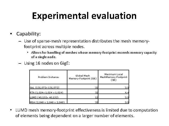
Experimental evaluation • Capability: – Use of sparse-mesh representation distributes the mesh memoryfootprint across multiple nodes. • Allows for handling of meshes whose memory-footprint exceeds memory capacity of a single node. – Using 16 nodes on Gig. E: Problem Instance Global Mesh Memory-Footprint (GB) Maximum Local Mesh. Memory-Footprint (GB) Go. L (131, 072 x 131, 072) 32 3. 0 RTA (1, 024 x 1, 024) 32 4. 4 LUMD (40, 132 x 40, 132) 12 3. 0 MSA (2, 048 x 2, 048) 32 3. 0 • LUMD mesh memory-footprint effectiveness is limited due to computation of elements being dependent on a larger number of elements.

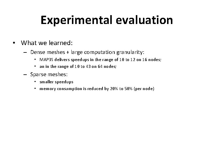
Experimental evaluation • What we learned: – Dense meshes + large computation granularity: • MAP 3 S delivers speedups in the range of 10 to 12 on 16 nodes; • an in the range of 10 to 43 on 64 nodes; – Sparse meshes: • smaller speedups • memory consumption is reduced by 20% to 50% (per node)

The End