The logic of Counterfactual Impact Evaluation 1 To

The logic of Counterfactual Impact Evaluation 1

To understand counterfactuals It is necessary to understand impacts

Impacts differ in one fundamental way from outputs and results Outputs and results are observable quantities

Can we observe an impact? No, we can’t

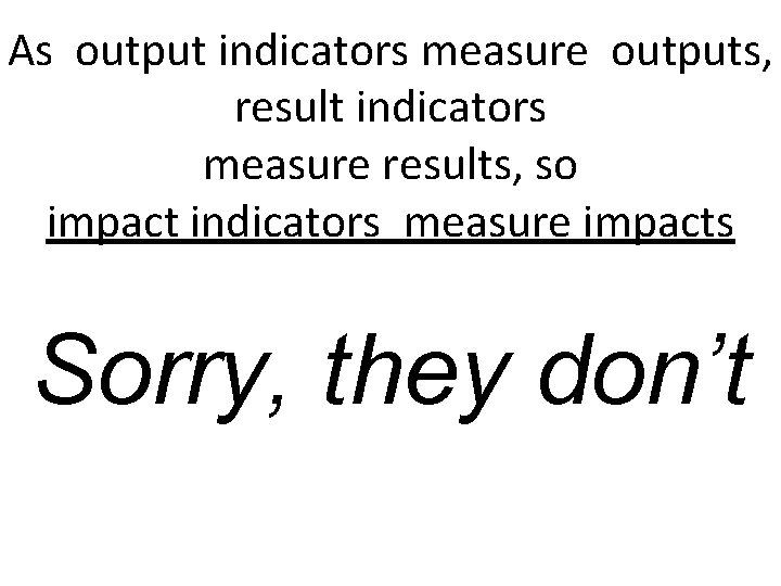
As output indicators measure outputs, result indicators measure results, so impact indicators measure impacts Sorry, they don’t

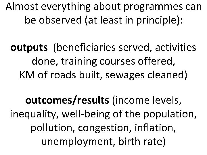
Almost everything about programmes can be observed (at least in principle): outputs (beneficiaries served, activities done, training courses offered, KM of roads built, sewages cleaned) outcomes/results (income levels, inequality, well-being of the population, pollution, congestion, inflation, unemployment, birth rate)

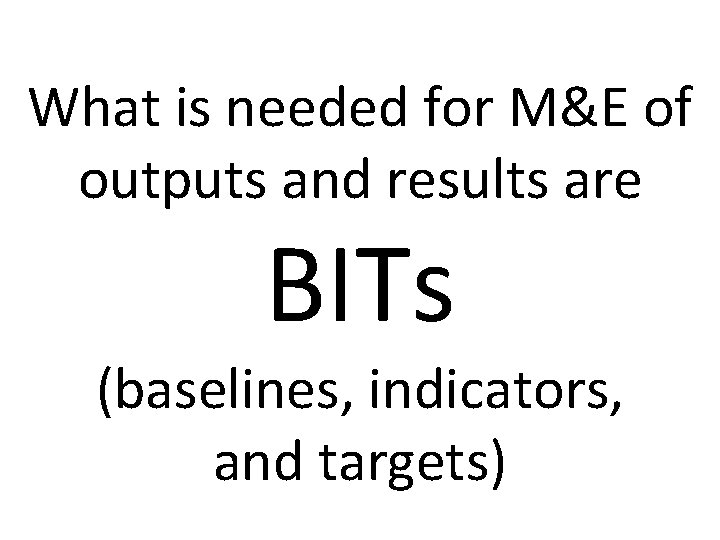
What is needed for M&E of outputs and results are BITs (baselines, indicators, and targets)

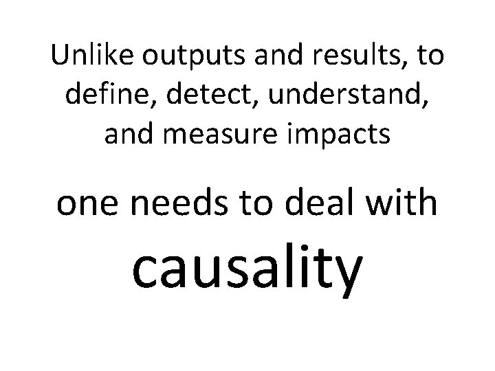
Unlike outputs and results, to define, detect, understand, and measure impacts one needs to deal with causality

“Causality is in the mind” J. J. Heckman

Why this focus on causality? Because, unless we can attribute changes (or differences) to policies, we do not know whether the intervention “works”, “for whom” it works, and even less “why” it works (or does not) Causal questions represents a bigger challenge than non causal questions (descriptive, normative, exploratory) 10

The social science scientific community defines impact/effect as “the difference between a situation observed after a stimulus has been applied and the situation that would have occurred without such stimulus” 11

A very intuitive example of the role of causality in producing credible evidence for policy decisions

Does playing chess have an impact on math learning?

Policy-relevant question: Should we make chess part of the regular curriculum in elementary schools, to improve mathematics achievement? Which kind of evidence do we need to make this decision in an informed way? We can think of three types of evidence, from the most naive to the most credible 14

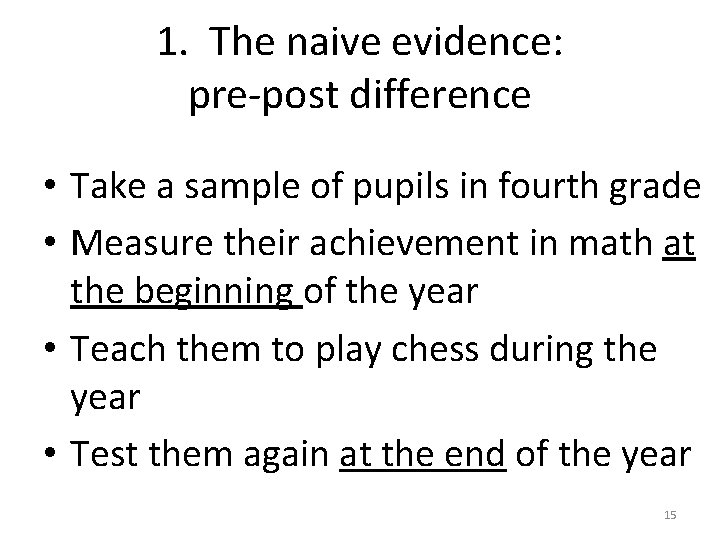
1. The naive evidence: pre-post difference • Take a sample of pupils in fourth grade • Measure their achievement in math at the beginning of the year • Teach them to play chess during the year • Test them again at the end of the year 15

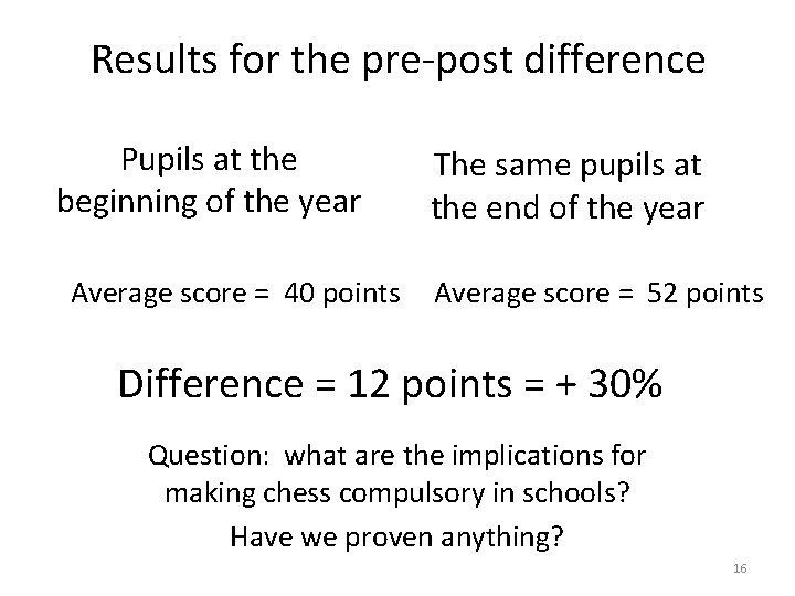
Results for the pre-post difference Pupils at the beginning of the year Average score = 40 points The same pupils at the end of the year Average score = 52 points Difference = 12 points = + 30% Question: what are the implications for making chess compulsory in schools? Have we proven anything? 16

Can we attribute the increase in test score to playing chess? OBVIOUSLY NOT The data tell us that the effect is between zero and 12 points • There is not doubt that many more factors are at play • So we must dismiss the increase in 10 points as unable to tell us anything about impact. 17

The pre-post great temptation • The pre-post comparisons have a great advantage: they seem kind of obvious (the “pop” definition of impact coincides with the pre-post difference) • Particularly when the intervention is big, and theory suggests that the outcomes should be affected • This is not the case here, but we should be careful in general to make causal inference based on pre-post comparisons 18

The risky alternative: with-without difference Compare math test scores for kids who have learned chess by themselves and kids who have not Impact = difference between treated and not treated? 19

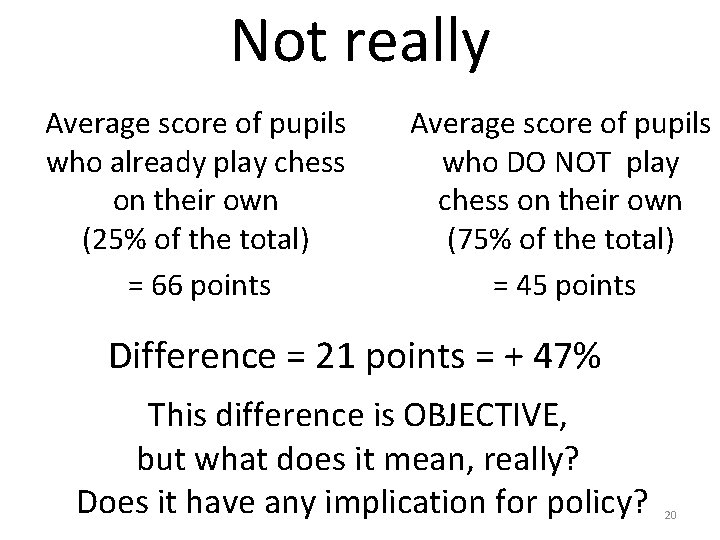
Not really Average score of pupils who already play chess on their own (25% of the total) = 66 points Average score of pupils who DO NOT play chess on their own (75% of the total) = 45 points Difference = 21 points = + 47% This difference is OBJECTIVE, but what does it mean, really? Does it have any implication for policy? 20

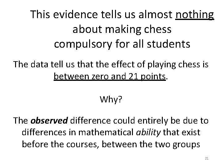
This evidence tells us almost nothing about making chess compulsory for all students The data tell us that the effect of playing chess is between zero and 21 points. Why? The observed difference could entirely be due to differences in mathematical ability that exist before the courses, between the two groups 21

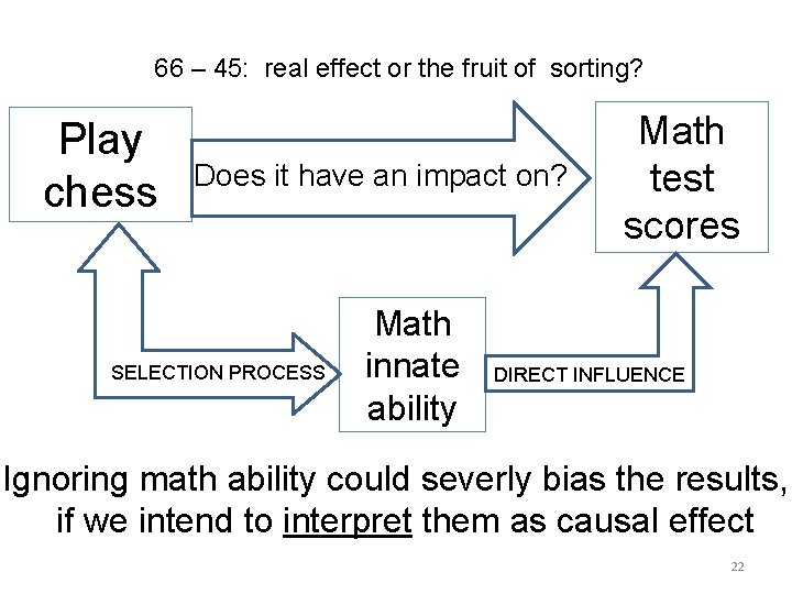
66 – 45: real effect or the fruit of sorting? Play chess Does it have. CSan impact on? SELECTION PROCESS Math innate ability Math test scores DIRDIRECT INFLUENCE Ignoring math ability could severly bias the results, if we intend to interpret them as causal effect 22

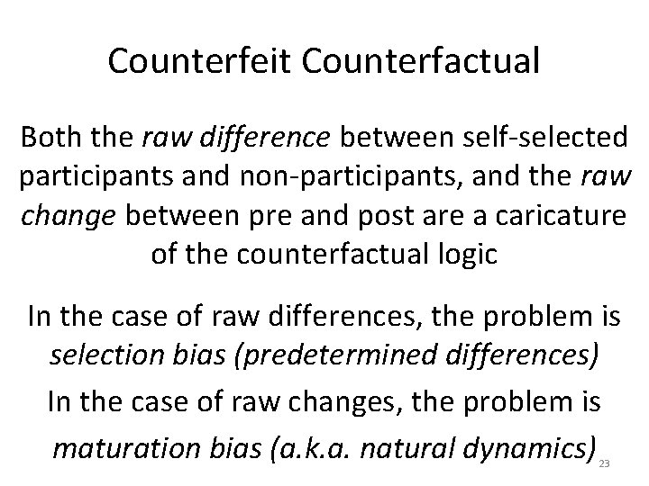
Counterfeit Counterfactual Both the raw difference between self-selected participants and non-participants, and the raw change between pre and post are a caricature of the counterfactual logic In the case of raw differences, the problem is selection bias (predetermined differences) In the case of raw changes, the problem is maturation bias (a. k. a. natural dynamics) 23

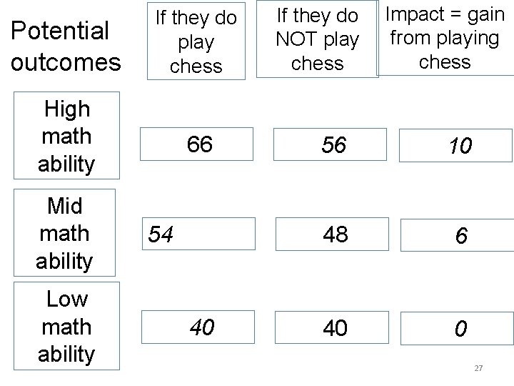
The modern way to understand causality is to think in terms of POTENTIAL OUTCOMES Let us imagine we know the score that kids would get if they played and they would get if they did not 24

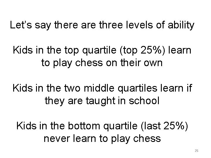
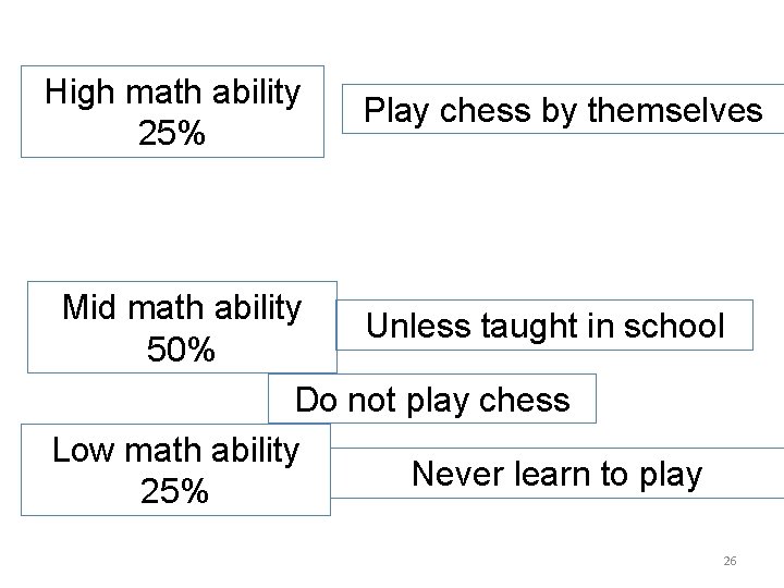
Let’s say there are three levels of ability Kids in the top quartile (top 25%) learn to play chess on their own Kids in the two middle quartiles learn if they are taught in school Kids in the bottom quartile (last 25%) never learn to play chess 25

High math ability 25% Play chess by themselves Mid math ability Unless taught in school 50% Do not play chess Low math ability Never learn to play 25% 26

Potential outcomes If they do play chess High math ability 66 Mid math ability Low math ability 54 40 If they do NOT play chess Impact = gain from playing chess 56 10 48 6 40 0 27

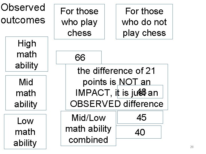
Observed outcomes High math ability Mid math ability Low math ability For those who play chess For those who do not play chess 66 the difference of 21 points is NOT an 48 an IMPACT, it is just OBSERVED difference Mid/Low math ability combined 45 40 28

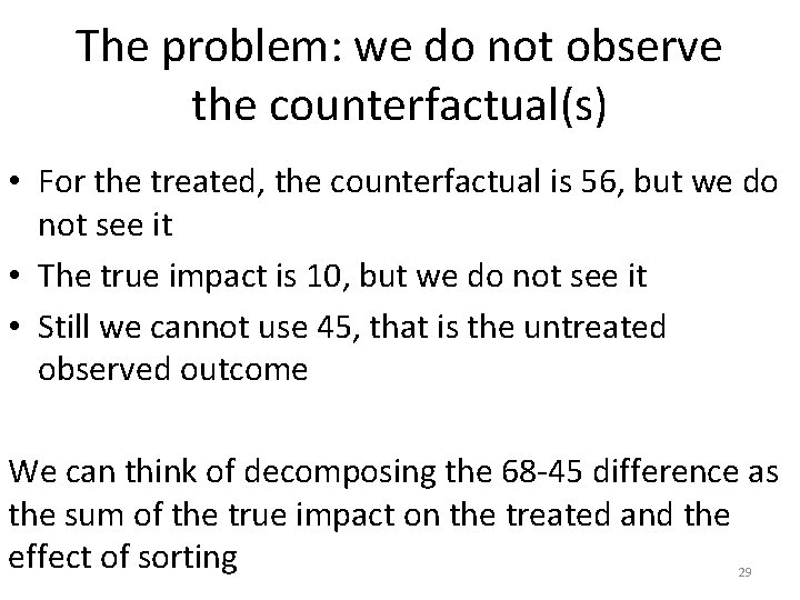
The problem: we do not observe the counterfactual(s) • For the treated, the counterfactual is 56, but we do not see it • The true impact is 10, but we do not see it • Still we cannot use 45, that is the untreated observed outcome We can think of decomposing the 68 -45 difference as the sum of the true impact on the treated and the effect of sorting 29

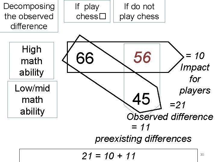
Decomposing the observed difference High math ability Low/mid math ability If play chess� 66 If do not play chess 56 45 = 10 Impact for players =21 Observed difference = 11 preexisting differences 21 = 10 + 11 30

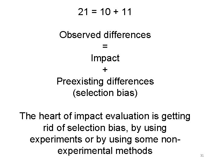
21 = 10 + 11 Observed differences = Impact + Preexisting differences (selection bias) The heart of impact evaluation is getting rid of selection bias, by using experiments or by using some nonexperimental methods 31

Experimental evidence to the rescue Schools get a free instructor to teach chess to one class, if they agree to select the class at random among the fourth grade classes Now we have the following situation 32

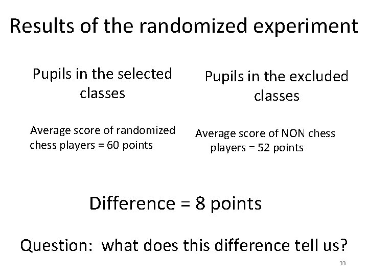
Results of the randomized experiment Pupils in the selected classes Average score of randomized chess players = 60 points Pupils in the excluded classes Average score of NON chess players = 52 points Difference = 8 points Question: what does this difference tell us? 33

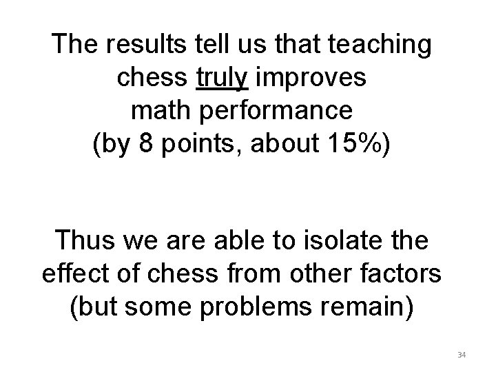
The results tell us that teaching chess truly improves math performance (by 8 points, about 15%) Thus we are able to isolate the effect of chess from other factors (but some problems remain) 34

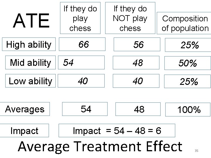
ATE If they do play chess High ability Mid ability Low ability Averages Impact 66 54 40 54 If they do NOT play chess Composition of population 56 25% 48 50% 40 25% 48 100% Impact = 54 – 48 = 6 Average Treatment Effect 35

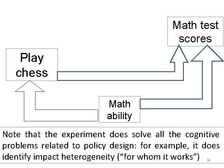
Math test scores Play chess DIRDIRE Math ability Note that the experiment does solve all the cognitive problems related to policy design: for example, it does identify impact heterogeneity (“for whom it works”) 36

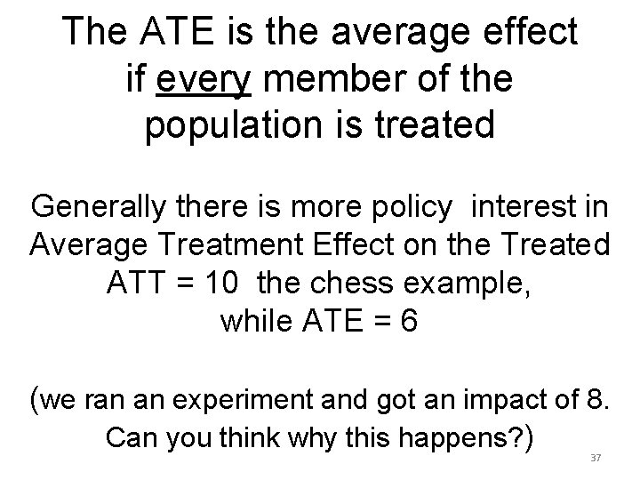
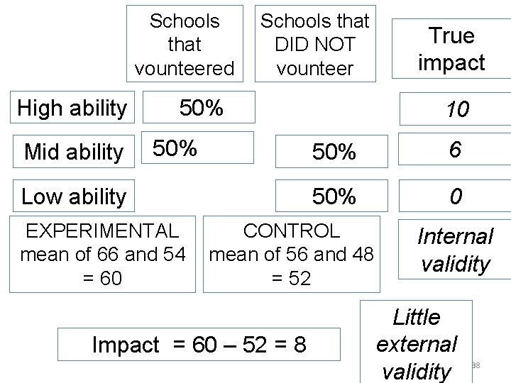
The ATE is the average effect if every member of the population is treated Generally there is more policy interest in Average Treatment Effect on the Treated ATT = 10 the chess example, while ATE = 6 (we ran an experiment and got an impact of 8. Can you think why this happens? ) 37

Schools that vounteered High ability Mid ability Schools that DID NOT vounteer 50% Low ability EXPERIMENTAL mean of 66 and 54 = 60 10 50% 6 50% 0 CONTROL mean of 56 and 48 = 52 Impact = 60 – 52 = 8 True impact Internal validity Little external validity 38

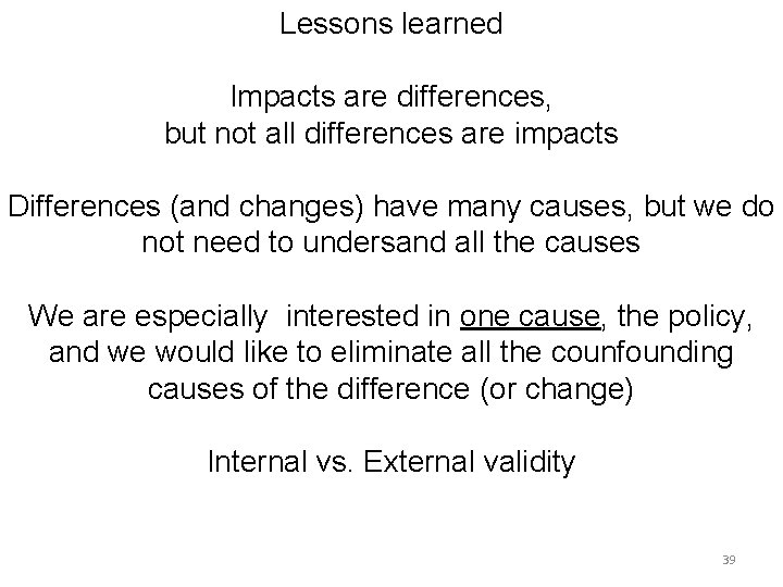
Lessons learned Impacts are differences, but not all differences are impacts Differences (and changes) have many causes, but we do not need to undersand all the causes We are especially interested in one cause, the policy, and we would like to eliminate all the counfounding causes of the difference (or change) Internal vs. External validity 39

An example of a real ERDF policy Grants to small enterprises to invest in R&D 40

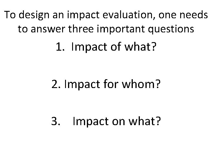
To design an impact evaluation, one needs to answer three important questions 1. Impact of what? 2. Impact for whom? 3. Impact on what?

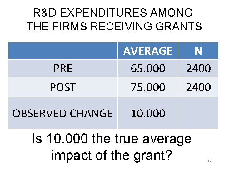
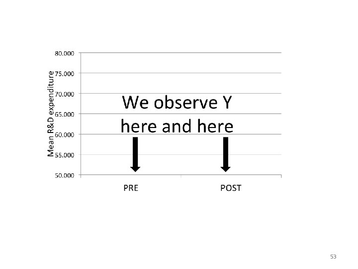
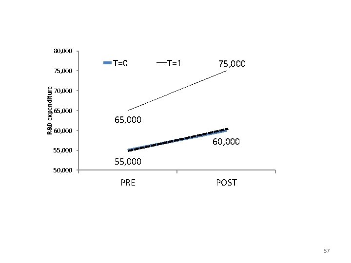
R&D EXPENDITURES AMONG THE FIRMS RECEIVING GRANTS PRE POST AVERAGE 65. 000 75. 000 OBSERVED CHANGE 10. 000 N 2400 Is 10. 000 the true average impact of the grant? 42

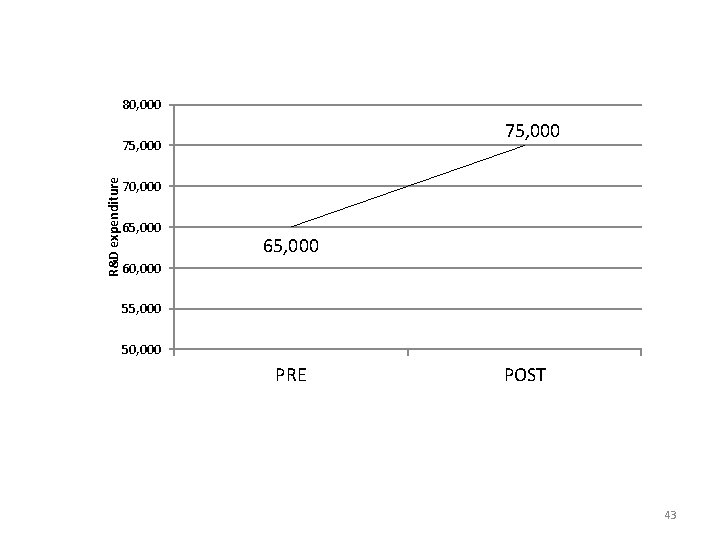
80, 000 75, 000 R&D expenditure 75, 000 70, 000 65, 000 60, 000 55, 000 50, 000 PRE POST 43

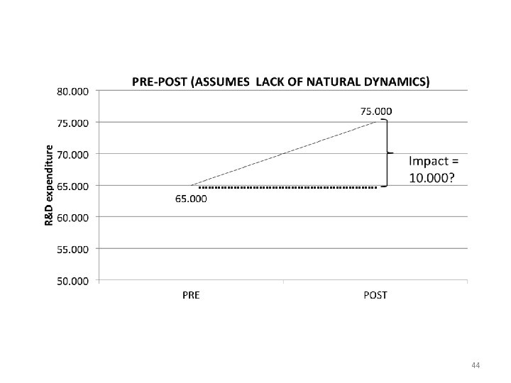
44

The fundamental challenge to this assumption is the well known fact that things change over time by “natural dynamics” How do we disentangle the change due to the policy from the myriad changes that would have occurred anyway? 45

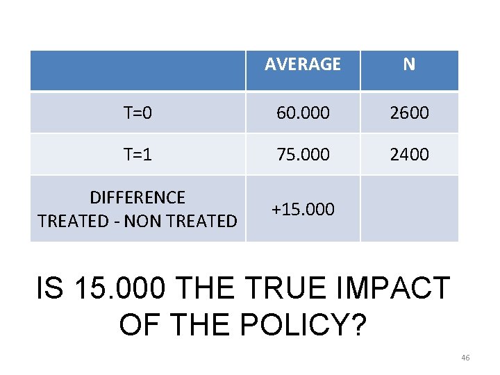
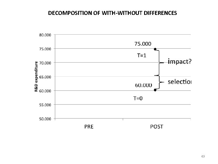
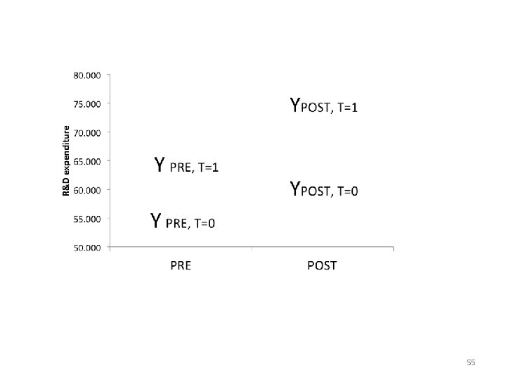
AVERAGE N T=0 60. 000 2600 T=1 75. 000 2400 DIFFERENCE TREATED - NON TREATED +15. 000 IS 15. 000 THE TRUE IMPACT OF THE POLICY? 46

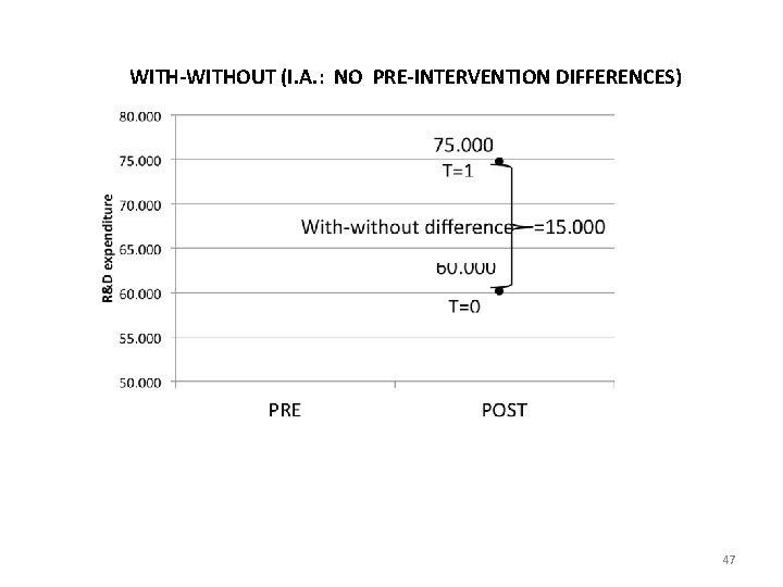
WITH-WITHOUT (I. A. : NO PRE-INTERVENTION DIFFERENCES) 47

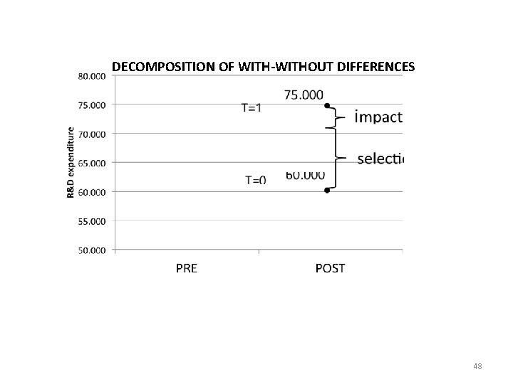
DECOMPOSITION OF WITH-WITHOUT DIFFERENCES 48

DECOMPOSITION OF WITH-WITHOUT DIFFERENCES 49

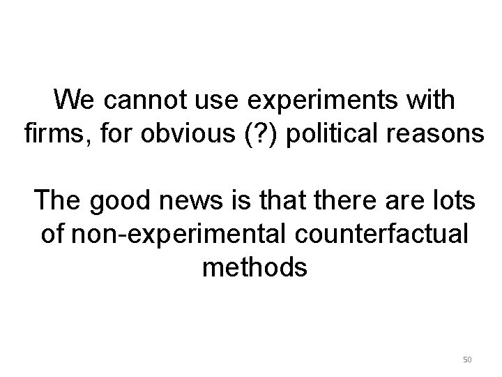
We cannot use experiments with firms, for obvious (? ) political reasons The good news is that there are lots of non-experimental counterfactual methods 50

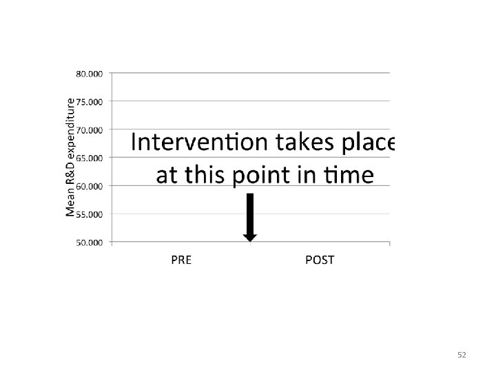
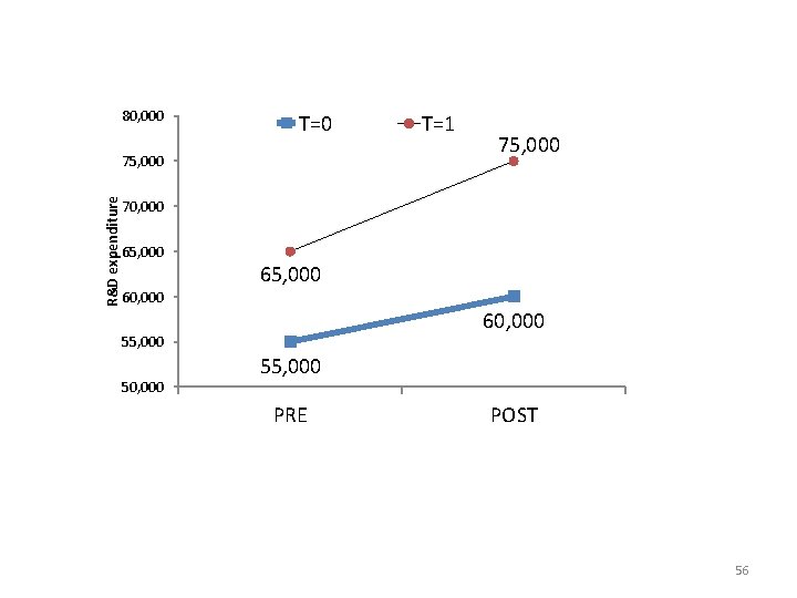
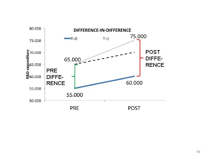
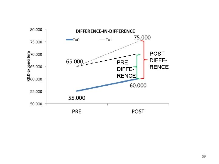
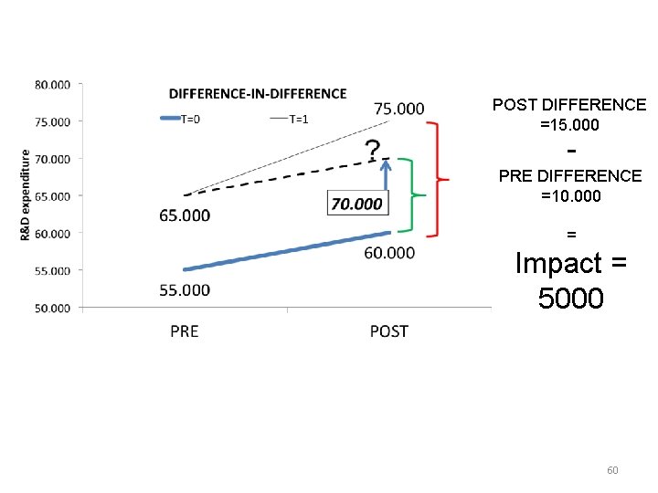
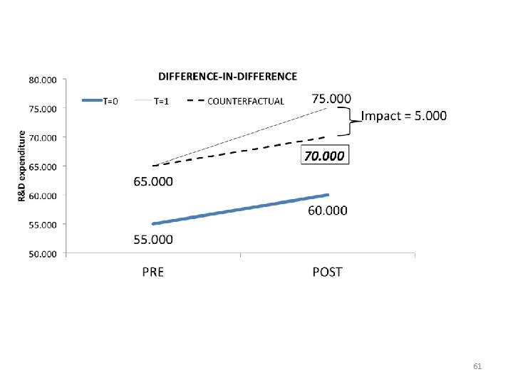
The difference-in-differences (DID) is a combination of the first two strategies And it is a good way to understand the logic of (non-experimental) counterfactual evaluation 51

52

53

54

55

80, 000 T=0 R&D expenditure 75, 000 T=1 75, 000 70, 000 65, 000 60, 000 55, 000 50, 000 55, 000 PRE POST 56

80, 000 R&D expenditure 75, 000 T=1 75, 000 70, 000 65, 000 60, 000 55, 000 50, 000 55, 000 PRE POST 57

PRE DIFFERENCE POST DIFFERENCE 58

PRE DIFFERENCE POST DIFFERENCE 59

POST DIFFERENCE =15. 000 - PRE DIFFERENCE =10. 000 = Impact = 5000 60

61

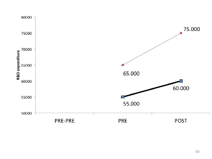
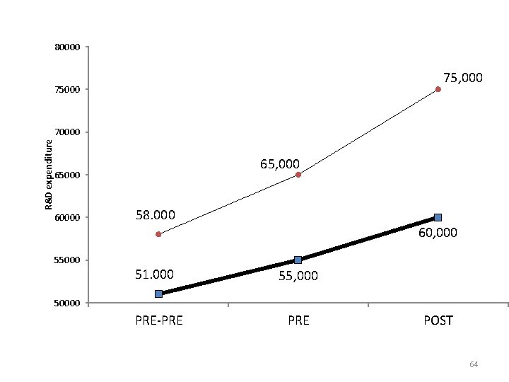
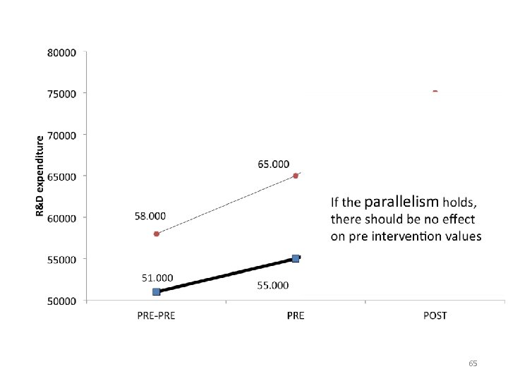
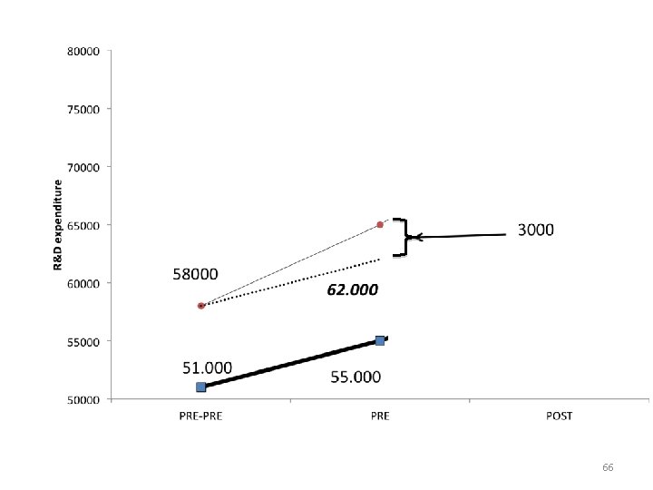
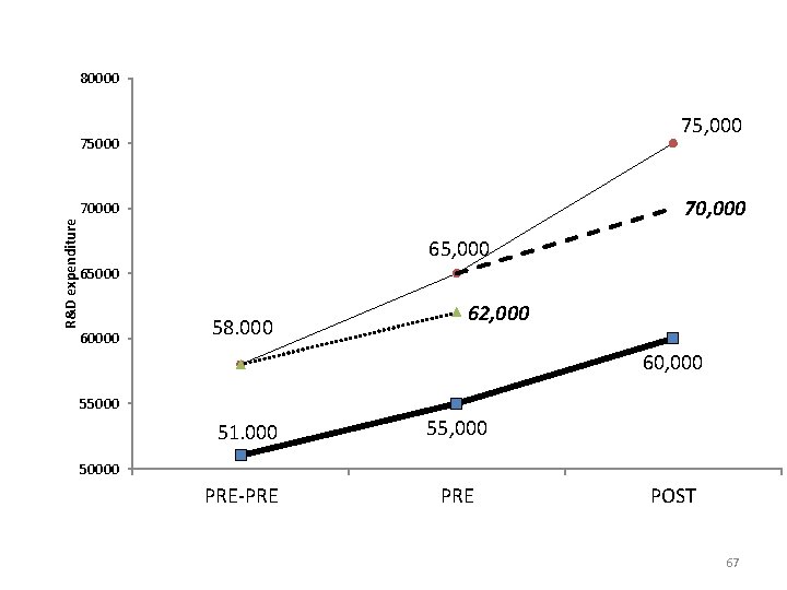
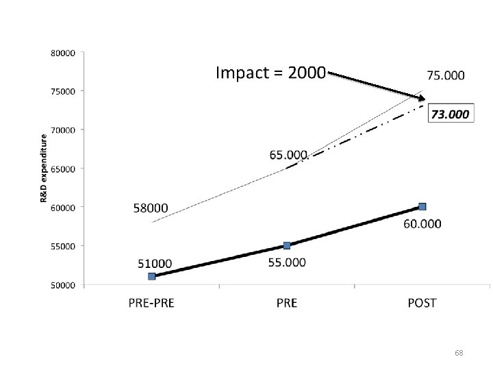
CAN WE TEST THE PARALLELISM ASSUMPTION? With four observed means, we cannot The parallelism becomes testable if we have two additional data points pre-intervention PRE-PRE 62

63

80000 75, 000 75000 R&D expenditure 70000 65, 000 65000 60000 58. 000 60, 000 55000 51. 000 55, 000 50000 PRE-PRE POST 64

65

66

80000 75, 000 75000 70, 000 R&D expenditure 70000 65, 000 65000 60000 58. 000 62, 000 60, 000 55000 51. 000 55, 000 PRE-PRE 50000 POST 67

68

WHEN TO USE DIFF-IN-DIFF? When we have longitudinal data and have reasons to believe that most of what drives selection is individual unobserved characteristics 69

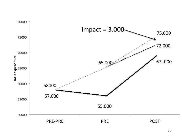
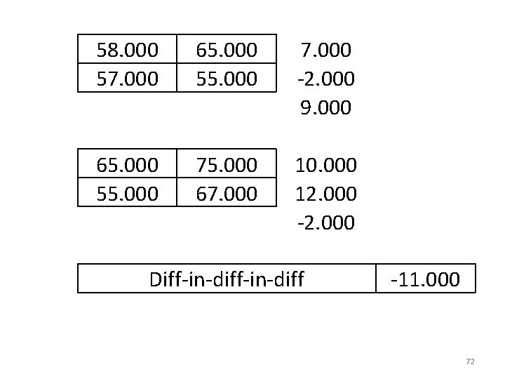
Second, the path taken by the controls must be a plausible approximation of what would happen to the treated The following is an example in which it would be better NOT to use DID 70

71

58. 000 57. 000 65. 000 55. 000 7. 000 -2. 000 9. 000 65. 000 55. 000 75. 000 67. 000 10. 000 12. 000 -2. 000 Diff-in-diff -11. 000 72

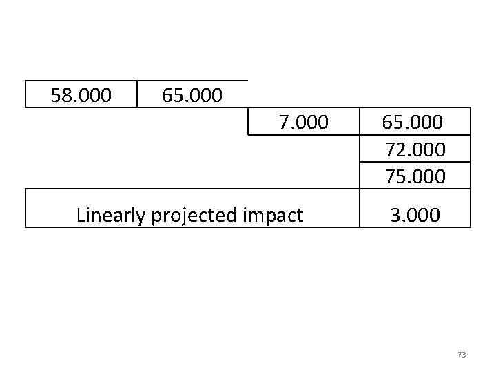
58. 000 65. 000 7. 000 Linearly projected impact 65. 000 72. 000 75. 000 3. 000 73