The largest possible gaps between quantum and classical

The largest possible gaps between quantum and classical algorithms Andris Ambainis University of Latvia Joint work with: Scott Aaronson, Kaspars Balodis, Aleksandrs Belovs, Troy Lee, Miklos Santha, and Juris Smotrovs

Quantum vs. classical k quantum steps How many steps classically?

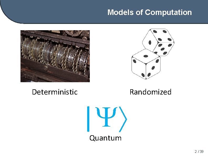
Models of Computation Deterministic Randomized | Quantum 2 / 39

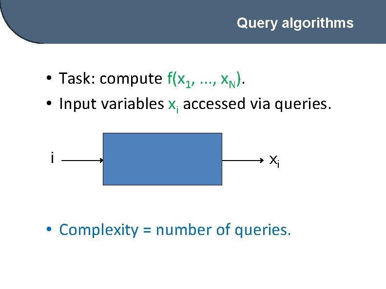
Query algorithms • Task: compute f(x 1, . . . , x. N). • Input variables xi accessed via queries. i xi • Complexity = number of queries.

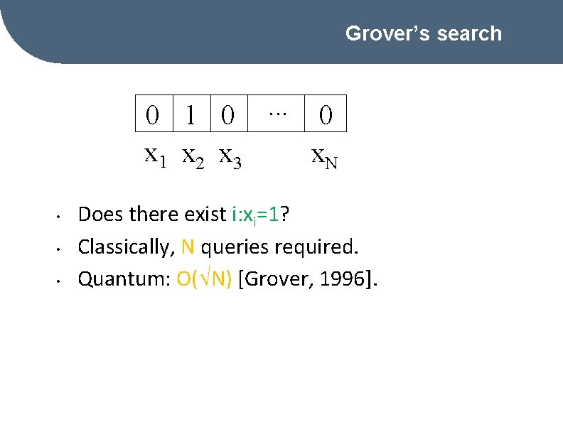
Grover’s search 0 1 0. . . 0 x 1 x 2 x 3 x. N • • • Does there exist i: xi=1? Classically, N queries required. Quantum: O( N) [Grover, 1996].

Reasons to study query model • Encompasses many quantum algorithms (Grover’s search, quantum part of factoring, etc. ). • Provable quantum-vs-classical gaps.

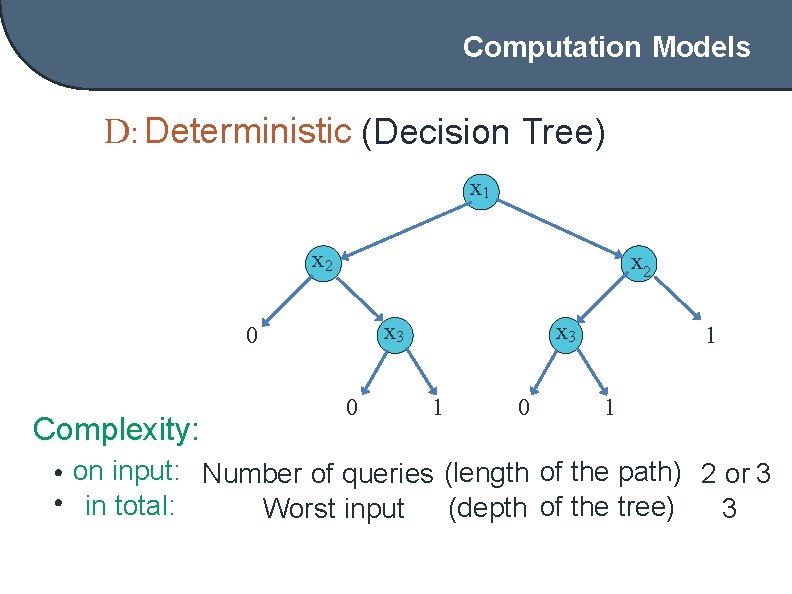
Computation Models D: Deterministic (Decision Tree) x 1 x 2 x 3 0 Complexity: 0 x 3 1 0 1 1 • on input: Number of queries (length of the path) 2 or 3 • in total: (depth of the tree) Worst input 3

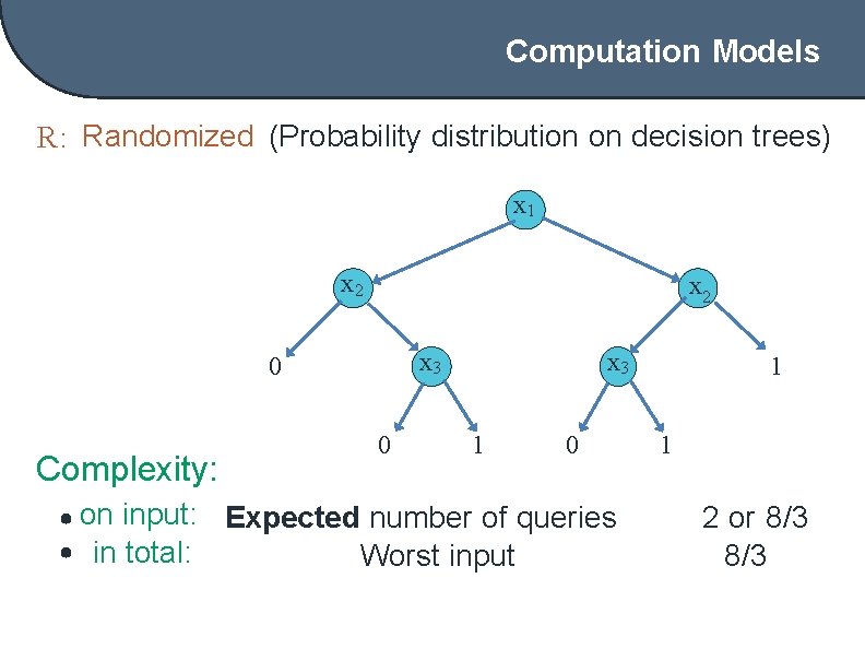
Computation Models R: Randomized (Probability distribution on decision trees) x 1 x 2 x 3 0 Complexity: • on input: • in total: 0 x 3 1 0 Expected number of queries Worst input 1 1 2 or 8/3

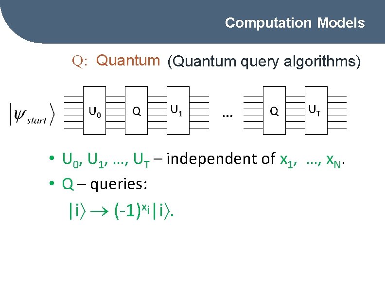
Computation Models Quantum query model Q: Quantum (Quantum query algorithms) U 0 Q U 1 … Q UT • U 0, U 1, …, UT – independent of x 1, …, x. N. • Q – queries: |i (-1)xi|i.

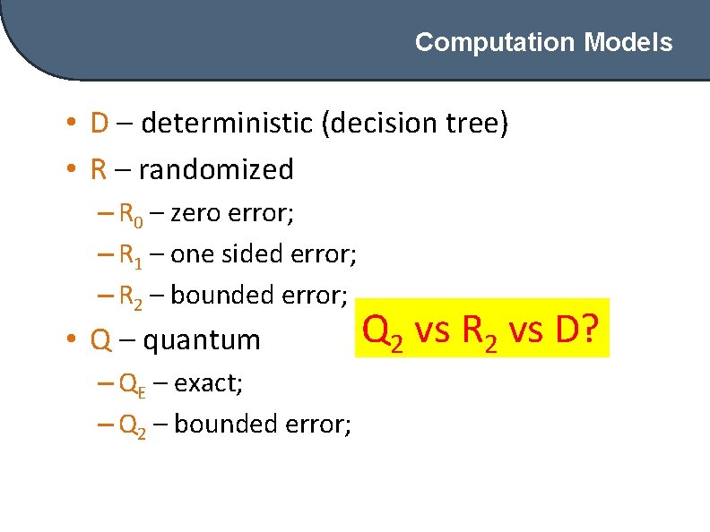
Computation Models • D – deterministic (decision tree) • R – randomized – R 0 – zero error; – R 1 – one sided error; – R 2 – bounded error; • Q – quantum – QE – exact; – Q 2 – bounded error; Q 2 vs R 2 vs D?

Settings • Partial functions: – For some inputs (x 1, . . . , x. N), the algorithm is allowed to output anything. – Huge quantum speedups. • Total functions: – Prescribed anwer f(x 1, . . . , x. N) for every (x 1, . . . , x. N). – Biggest quantum speedup: Grover.

Partial functions

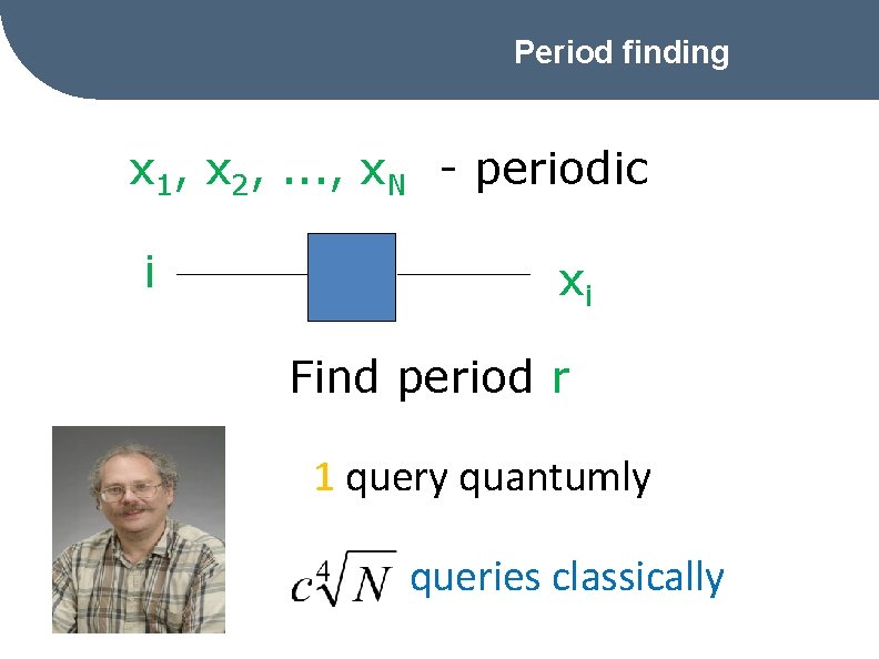
Period finding x 1, x 2, . . . , x. N - periodic i xi Find period r 1 query quantumly queries classically

Our result [Aaronson, A] • Task that requires 1 query quantumly, ( N/log N) classically. • 1 query quantum algorithms can be simulated by O( N) query probabilistic algorithms.

FORRELATION = Fourier CORRELATION

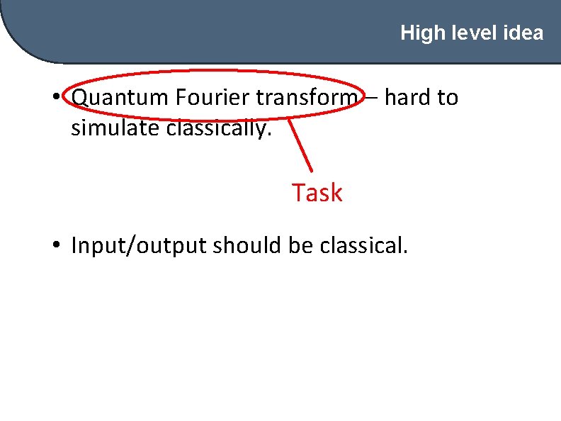
High level idea • Quantum Fourier transform – hard to simulate classically. Task • Input/output should be classical.

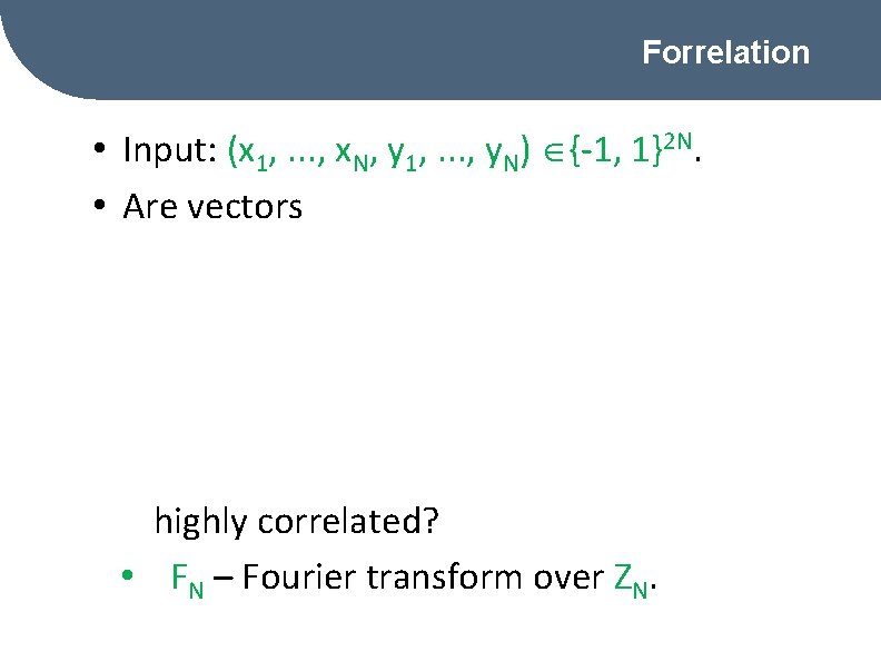
Forrelation • Input: (x 1, . . . , x. N, y 1, . . . , y. N) {-1, 1}2 N. • Are vectors highly correlated? • FN – Fourier transform over ZN.

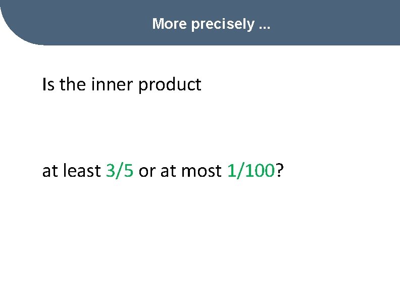
More precisely. . . Is the inner product at least 3/5 or at most 1/100?

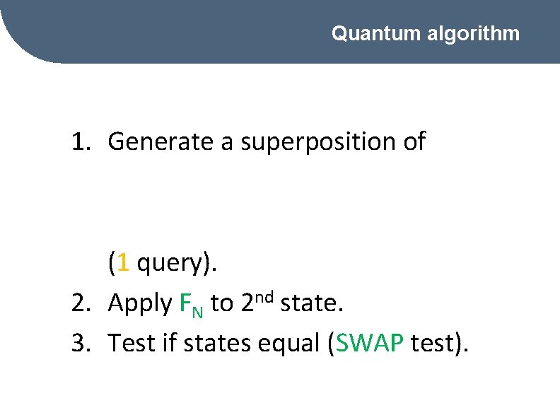
Quantum algorithm 1. Generate a superposition of (1 query). 2. Apply FN to 2 nd state. 3. Test if states equal (SWAP test).

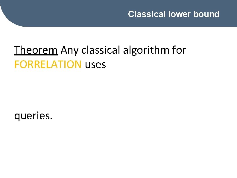
Classical lower bound Theorem Any classical algorithm for FORRELATION uses queries.

Simulating 1 query quantum algorithms

Simulation Theorem Any 1 query quantum algorithm can be simulated probabilistically with O( N) queries.

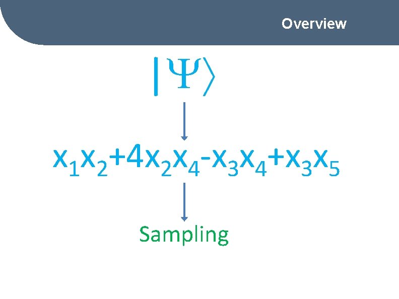
Overview | x 1 x 2+4 x 2 x 4 -x 3 x 4+x 3 x 5 Sampling

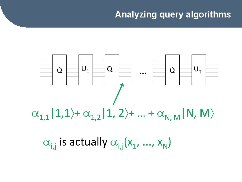
Analyzing query algorithms Q U 1 Q … Q UT 1, 1|1, 1 + 1, 2|1, 2 + … + N, M|N, M i, j is actually i, j(x 1, . . . , x. N)

Polynomials method Lemma [Beals et al. , 1998] After k queries, the amplitudes are polynomials in x 1, . . . , x. N of degree k. Measurement: Polynomial of degree 2 k

Our task • Pr[A outputs 1] = p(x 1, . . . , x. N), deg p =2. • 0 p(x 1, . . . , x. N) 1. • Task: estimate p(x 1, . . . , x. N) with precision . Solution: random sampling.

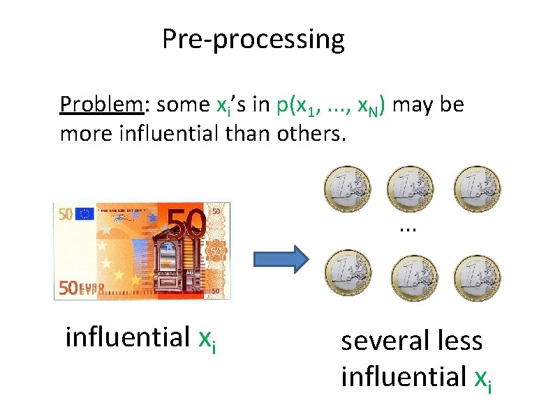
Pre-processing Problem: some xi’s in p(x 1, . . . , x. N) may be more influential than others. . influential xi several less influential xi

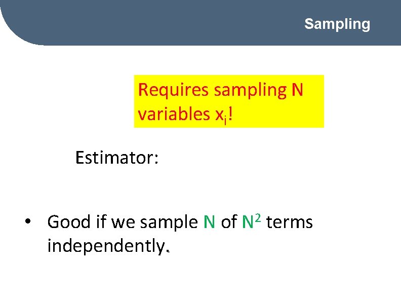
Sampling Requires sampling N variables xi! Estimator: • Good if we sample N of N 2 terms independently.

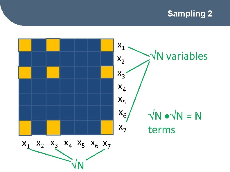
Sampling 2 x 1 x 2 x 3 x 4 x 5 x 6 x 7 N N variables N N = N terms

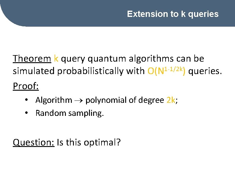
Extension to k queries Theorem k query quantum algorithms can be simulated probabilistically with O(N 1 -1/2 k) queries. Proof: • Algorithm polynomial of degree 2 k; • Random sampling. Question: Is this optimal?

k-fold forrelation

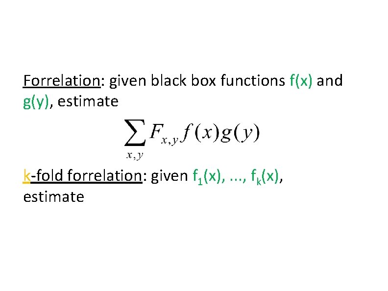
Forrelation: given black box functions f(x) and g(y), estimate k-fold forrelation: given f 1(x), . . . , fk(x), estimate

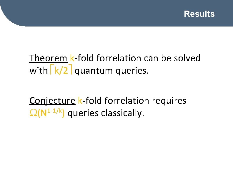
Results Theorem k-fold forrelation can be solved with k/2 quantum queries. Conjecture k-fold forrelation requires (N 1 -1/k) queries classically.

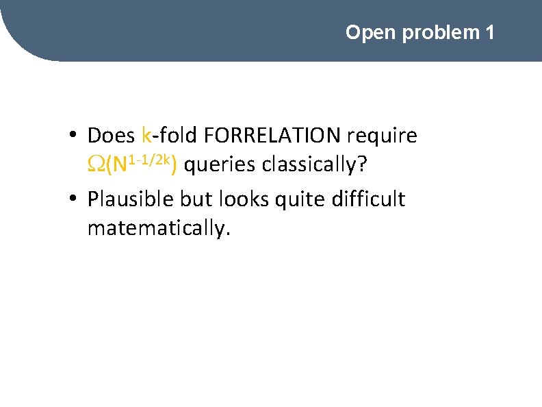
Open problem 1 • Does k-fold FORRELATION require (N 1 -1/2 k) queries classically? • Plausible but looks quite difficult matematically.

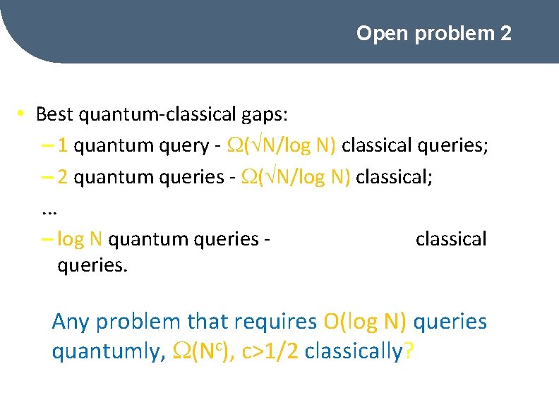
Open problem 2 • Best quantum-classical gaps: – 1 quantum query - ( N/log N) classical queries; – 2 quantum queries - ( N/log N) classical; . . . – log N quantum queries classical queries. Any problem that requires O(log N) queries quantumly, (Nc), c>1/2 classically?

Total functions

Why total functions? Partial functions: – huge quantum advantages. . . – achieved by ignoring the inputs where quantum algorithm does not provide a conclusive answer. What if the algorithm has to output a conclusive answer for every (x 1, . . . , x. N)?

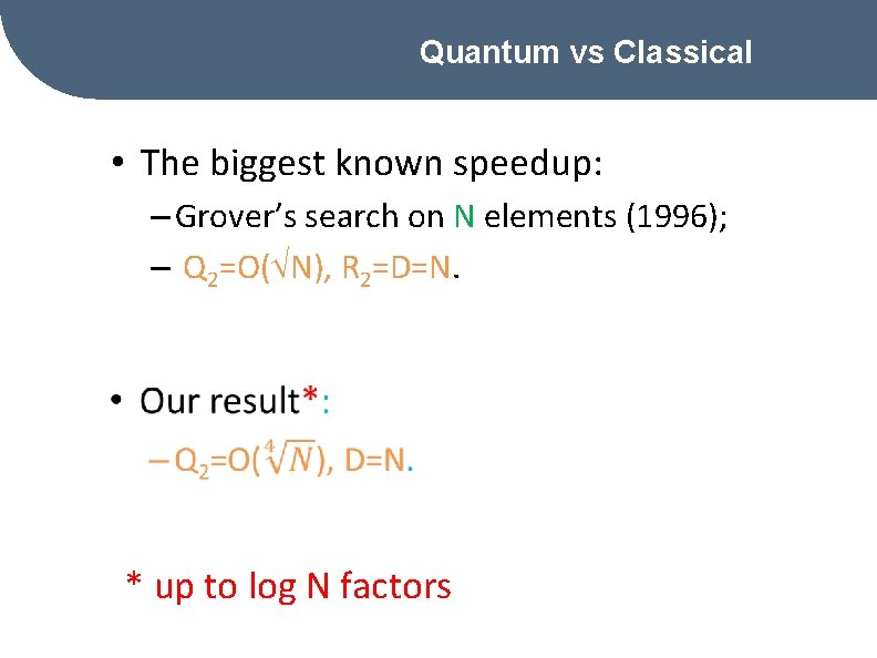
Quantum vs Classical • The biggest known speedup: – Grover’s search on N elements (1996); – Q 2=O( N), R 2=D=N. * up to log N factors

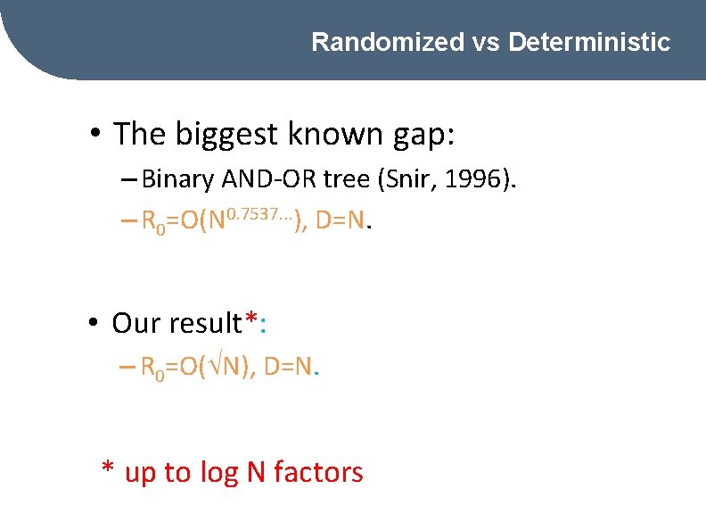
Randomized vs Deterministic • The biggest known gap: – Binary AND-OR tree (Snir, 1996). – R 0=O(N 0. 7537. . . ), D=N. • Our result*: – R 0=O( N), D=N. * up to log N factors

Two notes •

Go o s-Pitassi-Watson

Paper

Goal • Communication vs. Partition number. • f with following properties: – D – large; – f=1 can be certified by values for a small number of variables. – Certificates are unambiguous.

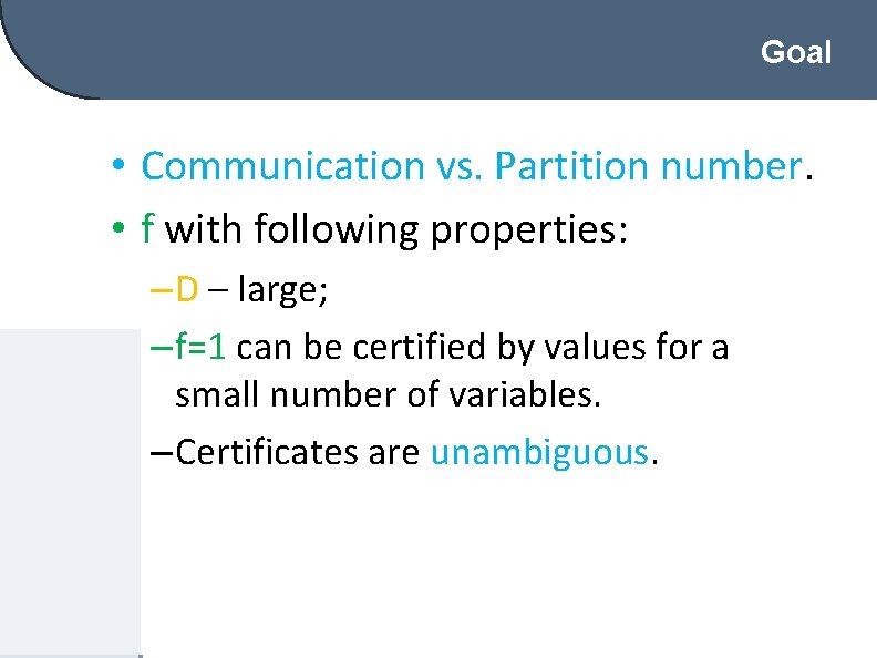
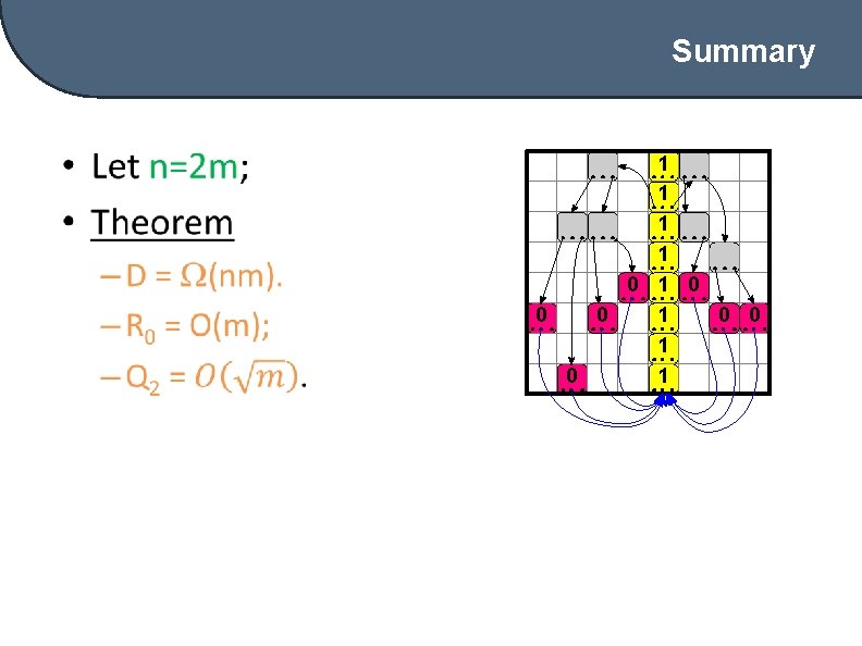
D versus 1 -certificates Function of nm variables f=1 iff there exists unique all-1 column 1 0 1 0 1 0 0 0 1 1 1 0 n D=nm m short 1 -certificates BUT not unambiguous.

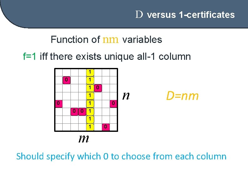
D versus 1 -certificates Function of nm variables f=1 iff there exists unique all-1 column 1 0 1 0 1 0 0 0 1 1 1 0 n D=nm m Should specify which 0 to choose from each column

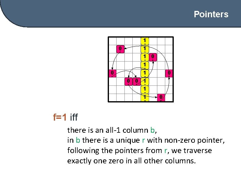
Pointers 1 0 1 0 1 0 0 0 1 1 1 0 f=1 iff there is an all-1 column b, in b there is a unique r with non-zero pointer, following the pointers from r, we traverse exactly one zero in all other columns.

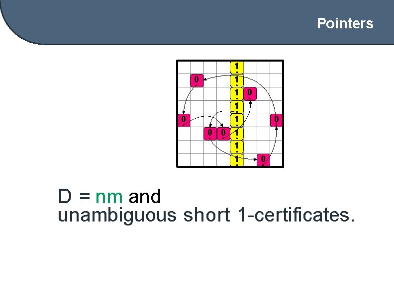
Pointers 1 0 1 0 1 0 0 0 1 1 1 0 D = nm and unambiguous short 1 -certificates.

Features Highly elusive (flexible) Still traversable (if know where to start).

Our Modifications

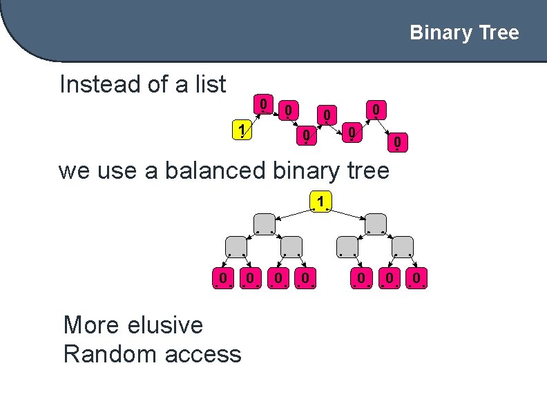
Binary Tree Instead of a list 0 0 1 0 0 0 we use a balanced binary tree 1 0 More elusive Random access 0 0 0

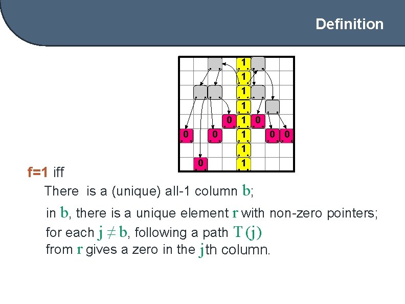
Definition f=1 iff 1 1 0 1 0 1 There is a (unique) all-1 column b; in b, there is a unique element r with non-zero pointers; for each j ≠ b, following a path T (j) from r gives a zero in the j th column.

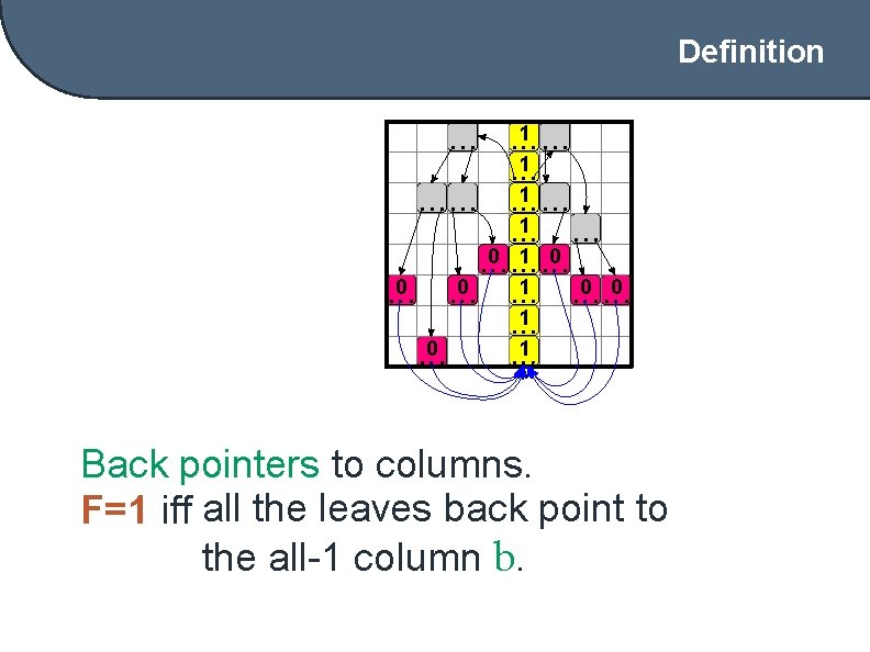
Definition 1 1 0 1 0 1 Back pointers to columns. F=1 iff all the leaves back point to the all-1 column b.

Q 2/R 0 versus D

Summary • 1 1 0 1 0 1

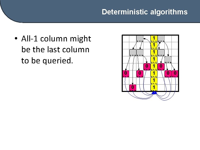
Deterministic algorithms • All-1 column might be the last column to be queried. 1 1 0 1 0 1

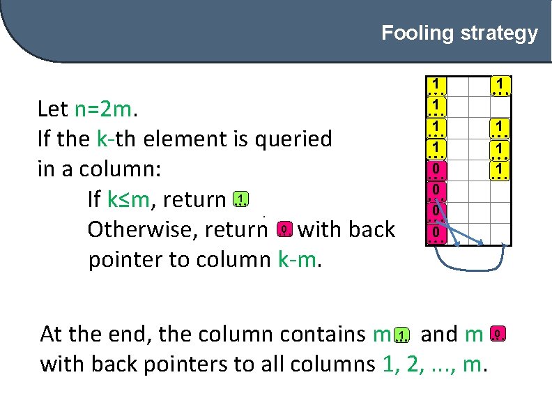
Fooling strategy Let n=2 m. If the k-th element is queried in a column: If k≤m, return 1. Otherwise, return 0 with back pointer to column k-m. 1 1 0 0 1 1 At the end, the column contains m 1 and m 0 with back pointers to all columns 1, 2, . . . , m.

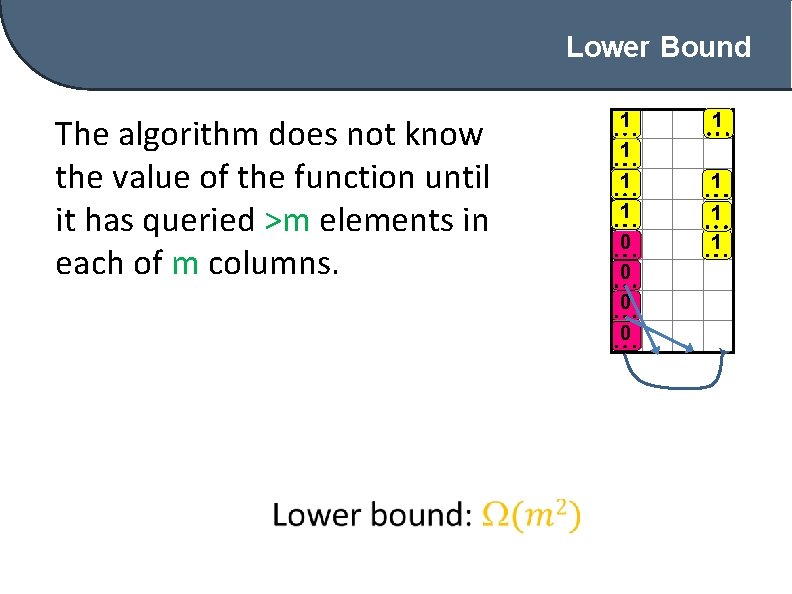
Lower Bound The algorithm does not know the value of the function until it has queried >m elements in each of m columns. 1 1 0 0 1 1

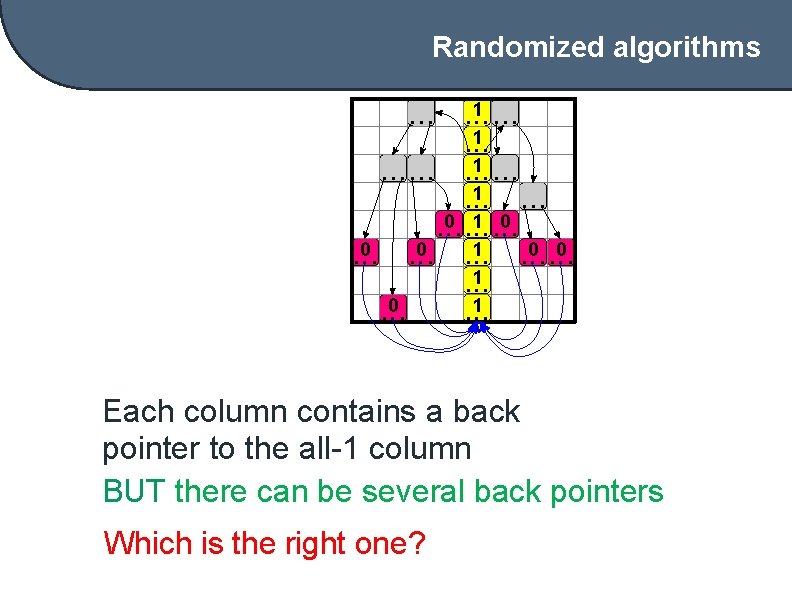
Randomized algorithms 1 1 0 1 0 1 Each column contains a back pointer to the all-1 column BUT there can be several back pointers Which is the right one?

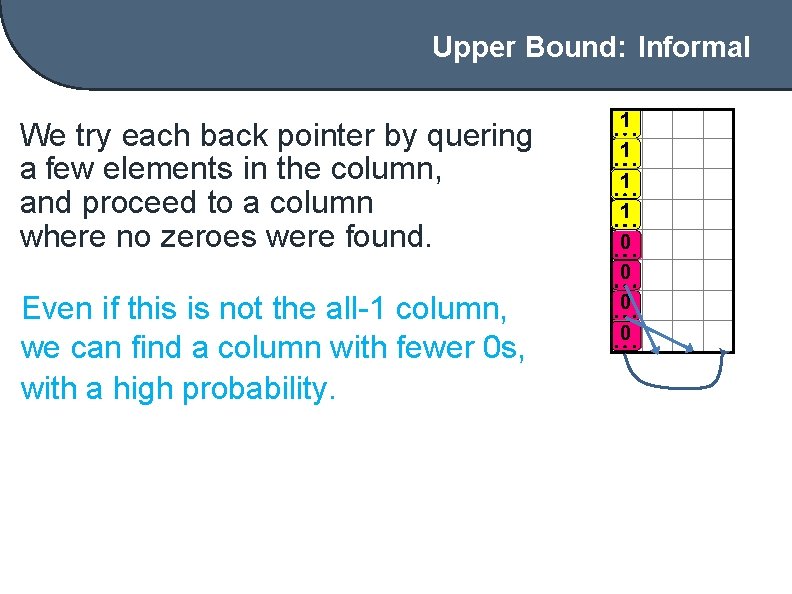
Upper Bound: Informal We try each back pointer by quering a few elements in the column, and proceed to a column where no zeroes were found. Even if this is not the all-1 column, we can find a column with fewer 0 s, with a high probability. 1 1 0 0

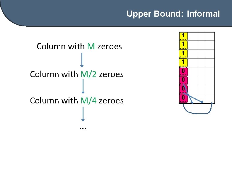
Upper Bound: Informal Column with M zeroes Column with M/2 zeroes Column with M/4 zeroes. . . 1 1 0 0

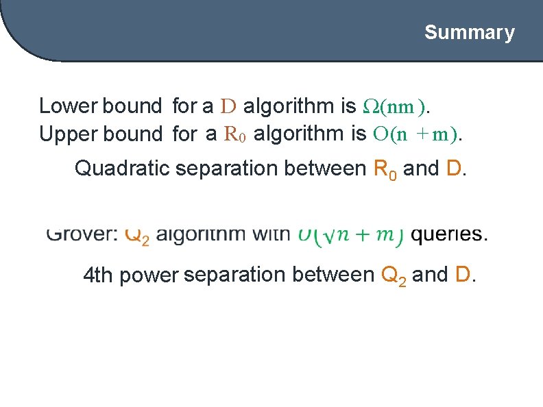
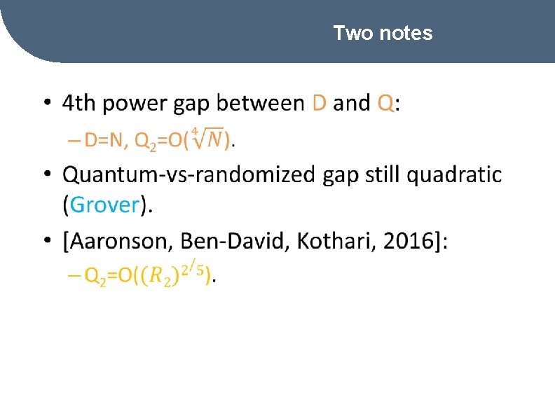
Summary Lower bound for a D algorithm is Ω(nm ). Upper bound for a R 0 algorithm is O (n + m). Quadratic separation between R 0 and D. 4 th power separation between Q 2 and D.

Other results

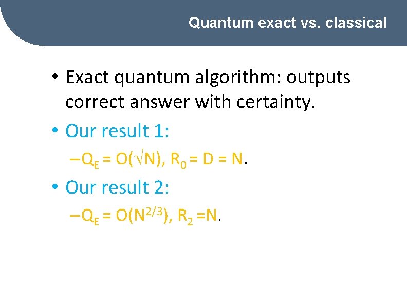
Quantum exact vs. classical • Exact quantum algorithm: outputs correct answer with certainty. • Our result 1: – QE = O( N), R 0 = D = N. • Our result 2: – QE = O(N 2/3), R 2 =N.

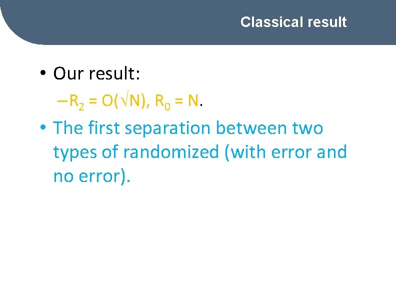
Classical result • Our result: – R 2 = O( N), R 0 = N. • The first separation between two types of randomized (with error and no error).

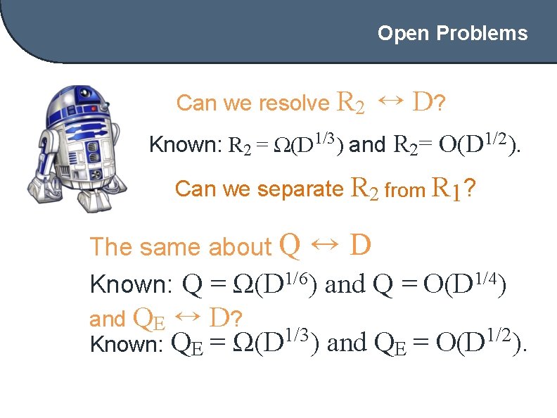
Open Problems Can we resolve R 2 ↔ D? Known: R 2 = Ω(D 1/3 ) and R 2= O(D 1/2). Can we separate R 2 from R 1? The same about Q ↔ D Known: Q = Ω(D 1/6) and Q = O(D 1/4) and QE ↔ D? Known: QE = Ω(D 1/3 ) and QE = O(D 1/2).

Any questions?