The Land Leverage Hypothesis Land leverage reflects the

The Land Leverage Hypothesis • Land leverage reflects the proportion of the total property value embodied in the value of the land (as distinct from improvements), as a significant factor for establishing the future path of property prices

The Land Leverage Hypothesis • It follows that the value of land value of improvements on that land are likely to evolve differently over time

The Land Leverage Hypothesis • Since total property price change is a weighted average of change in both land value and improvements, properties that vary in terms of how value is distributed between land improvements will show different price changes over time

The Land Leverage Hypothesis • The land leverage hypothesis suggests that the magnitude of price responses should be positively correlated to the level of land leverage

The Land Leverage Hypothesis • It will be demonstrated that changes in a property's overall value will depend critically on how much of the total value is contained in the land component • This proportion of total value comprised in the land component can be called "land leverage" • Bostic, W. , Longhofer, and S. D. , Redfearn, C. L. 2007. Land Leverage: Decomposing Home Price Dynamics. Real Estate Economics 35: 2: pp. 183 -208.

A general stylized example • • • Consider two homes, one located in Sydney and the other in Adelaide Both homes are valued at $450, 000 In Sydney, the $450, 000 home would likely be a lower-end home in an established area with older depreciated improvements Suppose that the improvements on the Sydney home are worth $90, 000 and the land is worth $360, 000 In Adelaide, however, the home is likely to be a higher-end home of new construction with an allocation of $360, 000 to improvements and $90, 000 to land value Assume that in a one year period, economic fundamentals (population, household growth, land supply, transportation costs etc) will cause land prices in both markets to increase by 10% during the year For simplicity, assume no depreciation associated with the housing structures and that construction costs remain stable The 10% increase in land prices will translate into a $36, 000 increase in the Sydney home, and the overall appreciation for the home would be 8% In contrast, the same 10% increase in land values will only result in a 2% increase in the value of the Adelaide home Despite the same magnitude of change in land prices, house prices in Sydney would appreciate four times faster than those in Adelaide

A general stylized example • In summary, the property in Sydney is highly land leveraged • High land leverage has a similar influence to financial leverage • Higher exposure to those factors influencing land prices within a local market will have a more significant influence with increasing land leverage • Land value becomes the major source of price appreciation and volatility • To illustrate this point, note that if economic fundamentals were to weaken so that land values dropped by 10%, it is the Sydney home that would suffer a larger overall decline in property value (- 8%), despite the fact that underlying land values changed by the same proportion in the two markets

Actual and Fundamental House Prices, Non-Fundamental Components and Interstate Spillovers: The Australian Experience. http: //ssrn. com/abstract=1460386

Data and Methodology

Data and Methodology

Data and Methodology

Data and Methodology

Data and Methodology

Empirical Tests of the Land Leverage Hypothesis • In order to calculate land leverage for an individual property, the value of the land must be identified separately from the value of the improvements

Empirical Tests of the Land Leverage Hypothesis • We do this by using a “market approach" in that we obtain market values of land improvements directly from observed sales

Empirical Tests of the Land Leverage Hypothesis • This is only possible for new construction, where the sale of a vacant lot can be identified prior to the sale of a completed home

Empirical Tests of the Land Leverage Hypothesis • i. iii. To be included in the sample an individual property must: have sold three times first as a vacant lot and then twice as a completed home • A further criterion was added in that the completed home must: i. have sold within two years of the vacant lot ii. and the final sale must have occurred at least one year after that • This one year restriction on the second sale is a guard against short -term speculative transactions being included in the sample

Empirical Tests of the Land Leverage Hypothesis

Structural Regression Results

Structural Regression Results

Structural Regression Results

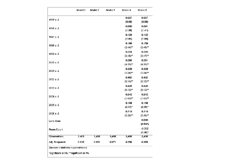
Reduced Form Regression Results • The advantage of the structural specification (equation 3) is that this model accurately accounts for different holding periods among individual properties in the sample • The main disadvantage is that it is very difficult to include and test other independent variables to check for stability of the model specification • It is intuitive that other factors such as the physical characteristics of an individual house, or time of sale, or location, may affect either land, or the building appreciation rate, and hence an individual properties overall appreciation rate • Table 4 provides results from various reduced form model specifications

Table 4 Results • Model 1 is a simple linear regression of initial land leverage on annualised growth (equation 2) • Results consistent with the more technically accurate nonlinear regression results, land values grow faster than building values • Model 2 includes the time between the vacant lot sale and the first sale (Time to resale) and the time between the two sales (Time to first sale), in years as independent variables • Time variables are highly significant, inclusion in the model lowers the estimated coefficients of the constant term and increases λ in the market sample • By definition, the time between the first and second improved sales (time to first sale) is also a proxy variable for the building age, capturing building depreciation hence influencing the constant term g. B

Table 4 Results • Model 3 introduces additional independent variables in the form of regional dummy variables interacting with land leverage • Assuming that construction costs should be generally equivalent throughout the Perth metropolitan region, location effects should only impact, g. L not g. B • Regional variables are included as interaction terms with the central and western regions serving as the omitted category (highest proportion of land leverage) • Land values have grown at different rates throughout the Perth metropolitan region - highly significant • Results should be treated with some caution as results to follow confirm some significant temporal patterns - time of the sale of vacant land could have a significant influence in some of these regions

Table 4 Results • Models 4 and 5 include independent variables interacting land leverage with a dummy variable for the year in which the vacant lot was purchased • 1988 -91 is the omitted category • The significant feature of these results is the impact on the overall land leverage variable λ • In models 4 and 5, where interacting time variables are included, the overall impact of land leverage, becomes insignificant at the marketwide level • However there are highly significant coefficients for a number of yearly periods • Significant temporal variation in the influence of land leverage • Most significant influence for land leverage is associated with vacant lot purchases in the later period of the sample 1998 -2006

Table 4 Results • Model 5 also introduces variables to test the influence of physical characteristics for individual properties • These variables are entered into the model directly (not interaction terms) • The size of an individual vacant lot is insignificant • Size of the building as measured by total rooms (room count) is slightly negative and statistically significant - also significant change in the constant term and in explanatory power for the model • Dependent variable in these regressions is the annualised growth in the property's value, the coefficients are interpreted as the impact on growth rates rather than the direct impact of these characteristics on home values • A negative coefficient on the size of the home (room count) implies that large homes have appreciated at a slower rate than have smaller homes

Conclusions • • • Results confirm the central proposition of the land leverage hypothesis Land values have increased at a faster rate than building values and homes and regions with high land leverage appreciated at a faster rate than those with lower land leverage Generally consistent with the Bostic et al. (2007) study In some respects results are significantly different from similar tests completed by Bostic et al. (2007) Significant temporal influences at work interacting with land leverage in the Perth housing market Temporal influences appear to be associated with boom market periods and rapid population increase in specific regions The influence of land leverage is not constant through time Results can be supplemented by extending the sample and methodology to incorporate established homes in addition to the market sample The land leverage hypothesis is an important emerging area of research with some important implications in understanding the price dynamics of urban regions, together with issues of housing affordability, town planning policy and the measurement of house price changes