The Importance of Understanding Type I and Type

The Importance of Understanding Type I and Type II Error in Statistical Process Control Charts – Continued Phillip R. Rosenkrantz, Ed. D. , P. E. California State Polytechnic University Pomona ASQ Orange Empire Section January 10, 2017 http: //www. cpp. edu/~rosenkrantz/prinfo/documents/asqdecisionrulescontd. pptx

2 Goals – Brief Review of Presentation-Part 1 in October 2016 n Brief review process control and process capability n Explain Type I and Type II error and give examples n Illustrate how the improper use of decision rules creates excessive Type I error and creates mistrust in SPC n Suggest simple approaches for reducing Type I error in SPC

3 Goals – Continued n Give examples of Type II error for common decision rules and available strategies for reducing Type II error. n Present some additional charts available to reduce Type II error for certain types of assignable causes n Educate about the common mistakes in industry related to using the wrong control chart. This mistake seems to more often increase Type II error (failure to detect) rather than Type I error (false alarm). n Discuss the proper use of Individuals charts.

4 Assignable vs. Common Cause Variation n Dr. Walter Shewhart developed Statistical Process Control (SPC) during the 1920 s. Dr. W. Edwards Deming promoted SPC during WWII and after. n Premise is that there are three types of variation n Common Cause Variation n Assignable (or Special Cause) variation n Tampering (or over-adjusting) n Each of these types of variation require a different approach or type of action.

5 Common Cause vs. Assignable Cause Variation n According to Dr. Deming’s research, more than 85% of problems are the result of “common cause” variation. Management is responsible for the system and it is their responsibility to work on reducing this type of variation. Later research puts the estimate at over 94%. n The work group is responsible for preventing and reducing “assignable cause” variation. n Management needs to understand these concepts.

6 Tampering – The Third Type of Variation n Tampering is over-adjusting the system caused by a lack of understanding of variation. n Sometimes large built in variation is mistaken for a process going “out of calibration” and needing adjustment n Over adjusting actually increases variation by adding more variation each time the process is changed n Tampering is a difficult habit to break because many machine operators consider it their “job” to constantly adjust their machine. n SPC reduces or eliminates unnecessary adjustments.

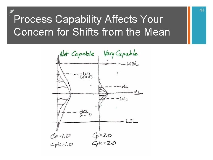
7 Major Concept #1: Process Capability n The ability of a process to produce within specification limits n Able to produce within specifications – process is “capable” n Not able to produce within specifications – “not capable” n Often quantified with process capability indices n Cp, Pp – Ability to stay within specs if centered n Cpk, Ppk – Ability based on current distribution

8 Major Concept #2: Process Control refers to how stable and consistent the process is. n “In-control” - stable and only experiencing systematic or “common cause” variation. n “Not in-control” – Process is not stable. Mean and variation are changing due to identifiable or “special” causes (usually controllable by those running the operation). n Represents <10% of the problems

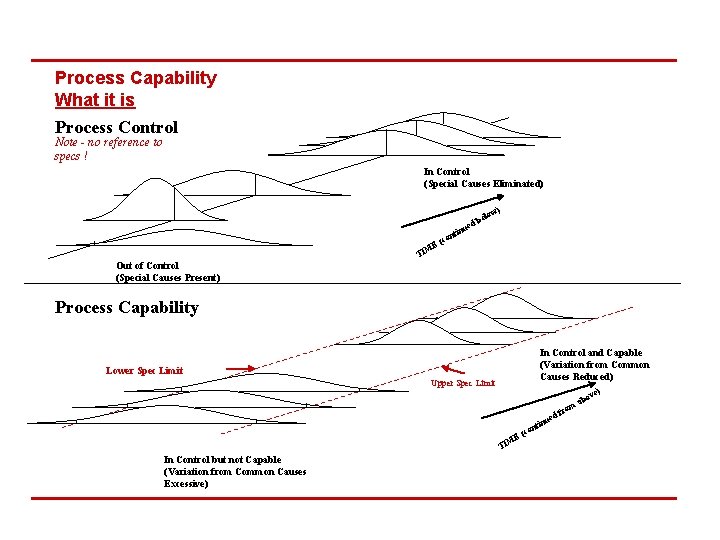
Process Capability What it is Process Control Note - no reference to specs ! In Control (Special Causes Eliminated) w) elo nti co E( b ued n M TI Out of Control (Special Causes Present) Process Capability In Control and Capable (Variation from Common Causes Reduced) Lower Spec Limit Upper Spec Limit t con ( ME TI In Control but not Capable (Variation from Common Causes Excessive) ed inu m fro ab ) ove

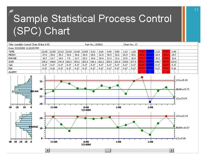
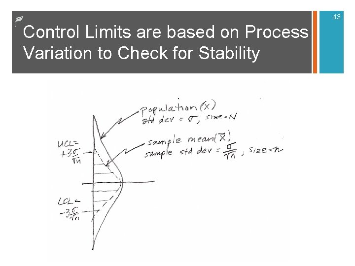
10 Control Charts n Walter Shewhart developed control charts that help management and workers identify common cause and special cause variation Management’s responsibility to reduce common cause variation n The work group is primarily responsible for controlling special or assignable cause variation n n Small samples are taken periodically with statistics (e. g. , average, range) plotted on charts and reveal the amount and type of variation. Control limits are traditionally +/- 3 standard deviations from the process average.

11 Sample Statistical Process Control (SPC) Chart

12 Use of Control Charts n. When the process remains within control limits with only a random pattern, process variation can be attributed to common cause variation (random variation in the system) and is deemed “in control. ” The process is stable and continues. n. When the process goes beyond control limits or is non-random, it is assumed that an assignable cause is present and deemed “out of control. ” The process is not stable and predictable. Find and eliminate the assignable cause.

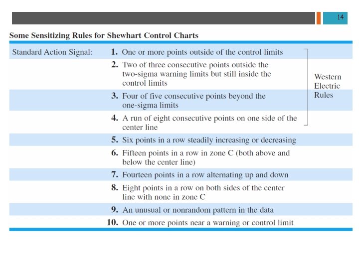
13 Decision or Sensitizing Rules n Decision Rules (a. k. a. Sensitizing rules) are used by operators to determine if a pattern of points indicates a process is no longer stable, that is: “out-of-control”. n Some rules are designed to detect changes or shifts in the process center (mean) n Some rules are designed to detect changes in the process variation (standard deviation) n Some rules are designed to detect a non-normal patterns (e. g. trends or cycles)

14

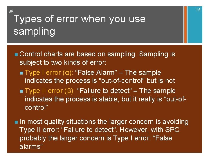
15 Types of error when you use sampling n Control charts are based on sampling. Sampling is subject to two kinds of error: n Type I error (α): “False Alarm” – The sample indicates the process is “out-of-control” but is not n Type II error (β): “Failure to detect” – The sample indicates the process is stable, but it really is “out-ofcontrol” n In most quality situations the larger concern is avoiding Type II error: “Failure to detect”. However, with SPC probably the larger concern is Type I error: “False alarms”

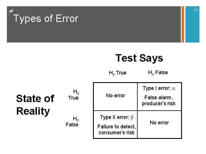
16 Types of Error Test Says H 0 True State of Reality H 0 True H 0 False H 0 False Type I error: a No error Type II error: b Failure to detect, consumer’s risk False alarm, producer’s risk No error

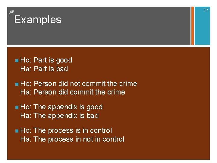
17 Examples n Ho: Part is good Ha: Part is bad n Ho: Person did not commit the crime Ha: Person did commit the crime n Ho: The appendix is good Ha: The appendix is bad n Ho: The process is in control Ha: The process in not in control

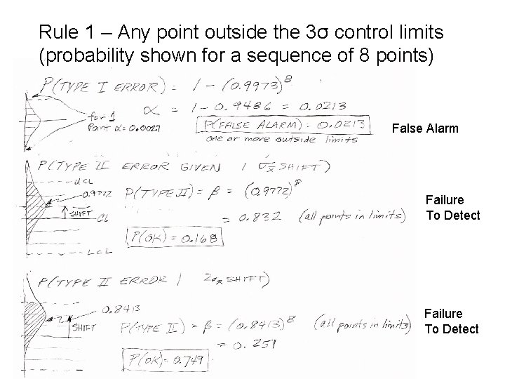
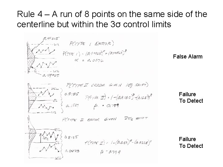
A look at two decision rules and the probability of Type I and Type II errors 18

Rule 1 – Any point outside the 3σ control limits (probability shown for a sequence of 8 points) False Alarm Failure To Detect

Rule 4 – A run of 8 points on the same side of the centerline but within the 3σ control limits False Alarm Failure To Detect

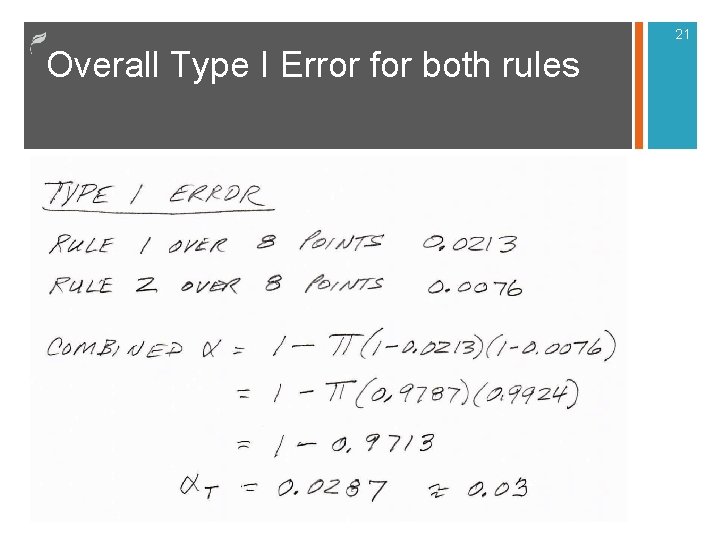
21 Overall Type I Error for both rules

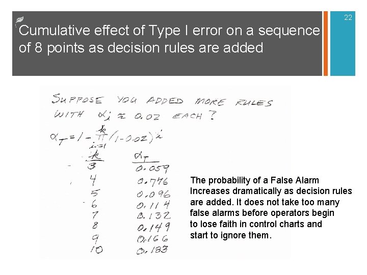
22 Cumulative effect of Type I error on a sequence of 8 points as decision rules are added The probability of a False Alarm Increases dramatically as decision rules are added. It does not take too many false alarms before operators begin to lose faith in control charts and start to ignore them.

23 Type I Error - A Common Problem That Makes SPC Ineffective n Too much Type I error eventually renders SPC ineffective. People get tired of chasing false alarms. n Many experts recommend using two decision rules (three at the most) to minimize Type I error. Rules 1 and 4 are commonly used. n Often, upon set up, software installers toggle on all decision rules thinking that is desirable. n If you use SPC software, ask to see which rules are in effect.

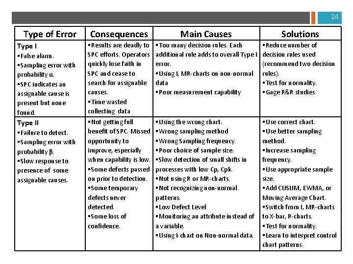
24 Type of Error Type I §False alarm. §Sampling error with probability α. §SPC indicates an assignable cause is present but none found. Type II §Failure to detect. §Sampling error with probability β. §Slow response to presence of some assignable causes. Consequences Main Causes Solutions §Results are deadly to SPC efforts. Operators quickly lose faith in SPC and cease to search for assignable causes. §Time wasted collecting data §Too many decision rules. Each additional rule adds to overall Type I error. §Using I, MR-charts on non-normal data §Poor measurement capability §Reduce number of decision rules used (recommend two decision rules). §Test for normality. §Gage R&R studies §Not getting full benefit of SPC. Missed opportunity to improve, especially when capability is low. §Some defects passed on prior to detection. §Some temporary defects never detected. §Some loss of confidence. §Using the wrong chart. §Wrong sampling method §Wrong Sampling frequency. §Poor choice of sample size. §Slow detection of small shifts in processes with low Cp, Cpk. §Not using R or MR-charts. §Not recognizing non-normal patterns. §Low Defect Level §Monitoring an attribute instead of a variable. §Using I-chart on Non-normal data. §Use correct chart. §Use better sampling method. §Increase sampling frequency. §Use appropriate sample size. §Add CUSUM, EWMA, or Moving Average Chart. §Switch from I, MR-charts to X-bar, R-charts. §Test for normality. §Learn to interpret control chart patterns.

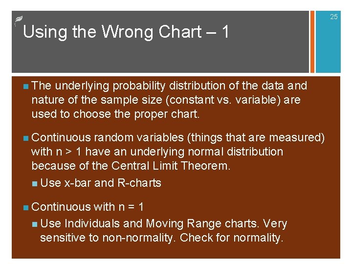
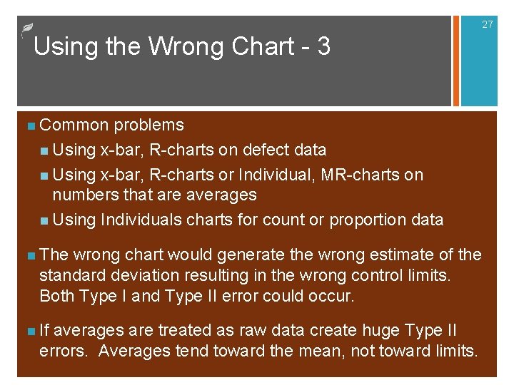
25 Using the Wrong Chart – 1 n The underlying probability distribution of the data and nature of the sample size (constant vs. variable) are used to choose the proper chart. n Continuous random variables (things that are measured) with n > 1 have an underlying normal distribution because of the Central Limit Theorem. n Use x-bar and R-charts n Continuous with n = 1 n Use Individuals and Moving Range charts. Very sensitive to non-normality. Check for normality.

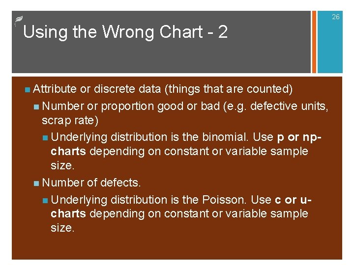
26 Using the Wrong Chart - 2 n Attribute or discrete data (things that are counted) n Number or proportion good or bad (e. g. defective units, scrap rate) n Underlying distribution is the binomial. Use p or npcharts depending on constant or variable sample size. n Number of defects. n Underlying distribution is the Poisson. Use c or ucharts depending on constant or variable sample size.

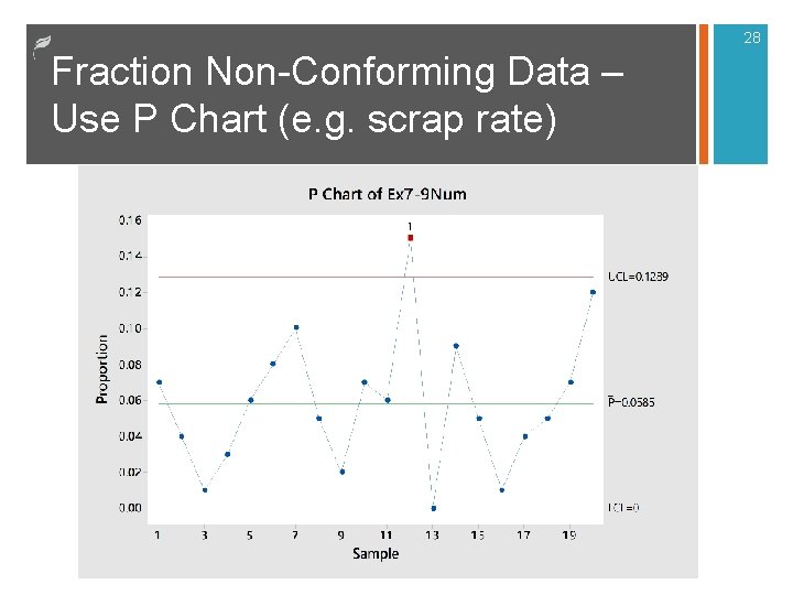
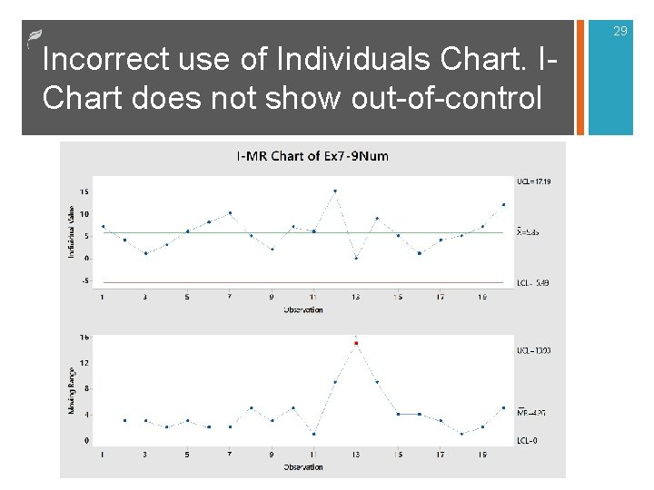
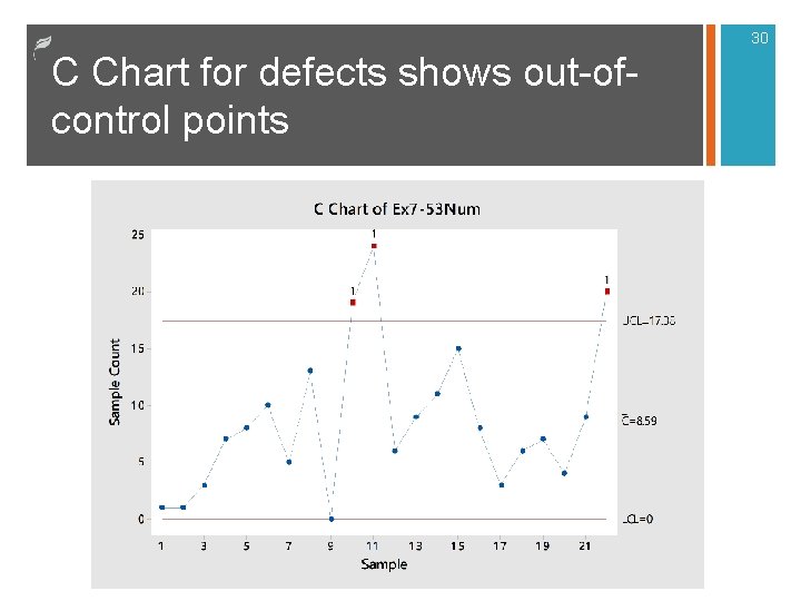
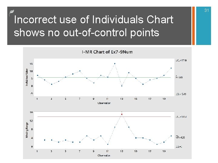
27 Using the Wrong Chart - 3 n Common problems n Using x-bar, R-charts on defect data n Using x-bar, R-charts or Individual, MR-charts on numbers that are averages n Using Individuals charts for count or proportion data n The wrong chart would generate the wrong estimate of the standard deviation resulting in the wrong control limits. Both Type I and Type II error could occur. n If averages are treated as raw data create huge Type II errors. Averages tend toward the mean, not toward limits.

28 Fraction Non-Conforming Data – Use P Chart (e. g. scrap rate)

29 Incorrect use of Individuals Chart. IChart does not show out-of-control

30 C Chart for defects shows out-ofcontrol points

31 Incorrect use of Individuals Chart shows no out-of-control points

32 Not using R-charts with x-bar charts n With normally distributed data the mean and standard deviation are statistically independent. Assignable cause could affect the mean (center), standard deviation (spread), or both. n Using only x-bar charts ignores assignable causes that affect variation. n Users need to be educated on why and how to use both charts together.

33 Using Individual (I) and Moving Range (MR) Charts n The Central Limit Theorm does not apply to individuals data so cannot assume normality. Need to check for normality. n MR method to determine standard deviation uses correlated (not independent) data which makes interpretation of the MR chart potentially invalid. Many experts do not trust the MR chart. n This can be a big problem resulting in either Type I or Type II error—depending on the underlying distribution. n Alternatives – Switch to x-bar, R-charts (n > 1) if practical, transform data, be wary of MR-chart patterns.

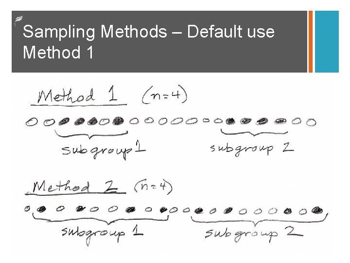
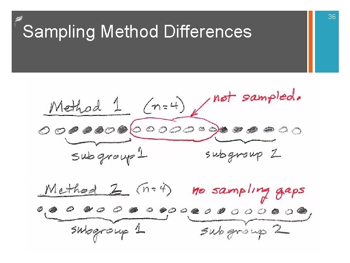
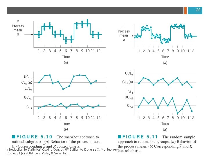
Wrong Sampling Method (a. k. a. Rational Subgrouping) - 1 n Method 1 – Snapshot approach. Samples taken at about the same time. Gap of time between samples. n Cheaper n Can miss assignable causes that come and go n Detects shifts in the sample mean faster n Method 2 – Random sample approach. Every unit has an equal chance of being in the sample. n Can be more labor intensive and therefore cost more n Less likely to miss causes that come and go n Less sensitive to detecting shifts in the sample mean 34

Sampling Methods – Default use Method 1

36 Sampling Method Differences

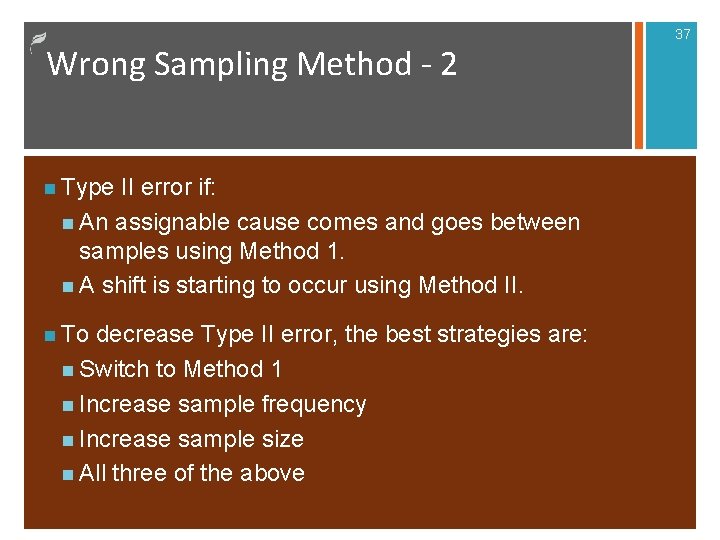
Wrong Sampling Method - 2 n Type II error if: n An assignable cause comes and goes between samples using Method 1. n A shift is starting to occur using Method II. n To decrease Type II error, the best strategies are: n Switch to Method 1 n Increase sample frequency n Increase sample size n All three of the above 37

38 Introduction to Statistical Quality Control, 6 th Edition by Douglas C. Montgomery. Copyright (c) 2009 John Wiley & Sons, Inc.

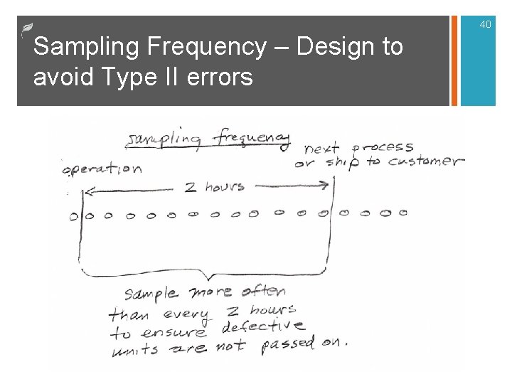
Wrong Sampling Frequency n If frequency between sampling is not close enough, an assignable cause can occur and make it through the process and out the door before detected. n Can end up with lots of defective product throughout the system. n Solution – Determine how long until a defective unit would get to a critical point would be expensive to correct. Sample frequency should be shortened to avoid bad product getting to that point. 39

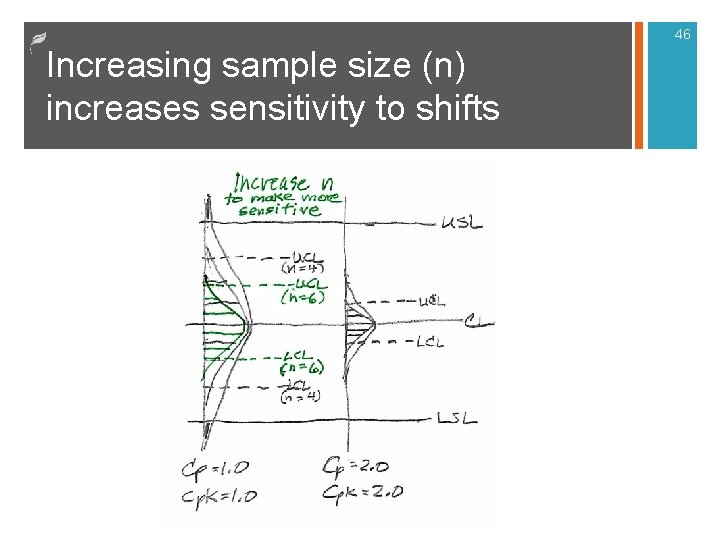
40 Sampling Frequency – Design to avoid Type II errors

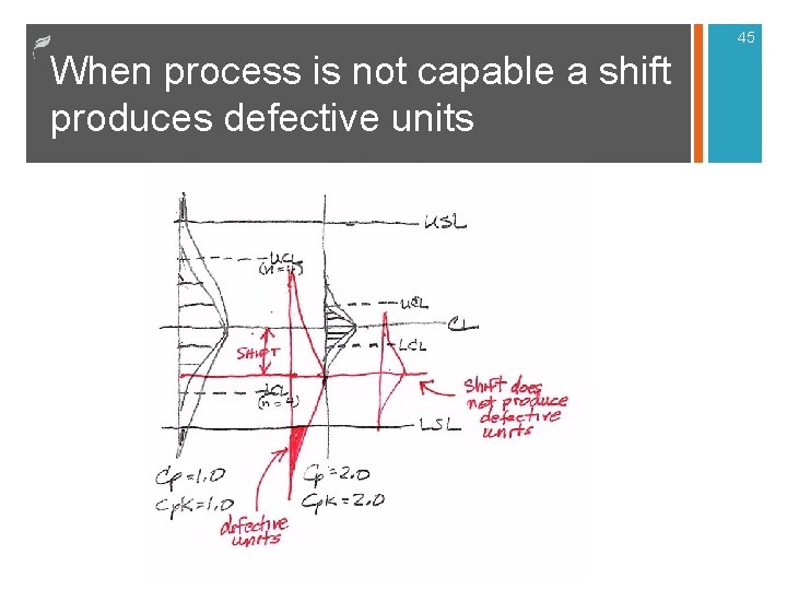
41 Poor Choice of Sample Size n Some companies always use the sample size for each application of x-bar and R-charts. (e. g. , always using n = 5) n Inceasing the sample size can be used to make charts more sensitive to shifts in the mean or increases in variation. n For processes that are very capable you can decrease n and save money. n For processes that are not capable, you need to increase n to protect against small shifts in the mean.

42 Failing to detect small shifts in low capability processes (Cp, Cpk ≤ 1. 67) n If Cp or Cpk are low, then small shifts can produce defective units. One weakness of the traditional Shewart control charts is in detecting small shifts in the mean— under 1 or 1. 5 standard deviations. n Can increase sample size and frequency to reduce Type II error. Added sampling can be expensive. n Alternative is to add a third chart that is specifically good at quickly detecting small shifts in the mean: Either the EWMA chart, CUSUM chart, or Moving Average chart.

43 Control Limits are based on Process Variation to Check for Stability

44 Process Capability Affects Your Concern for Shifts from the Mean

45 When process is not capable a shift produces defective units

46 Increasing sample size (n) increases sensitivity to shifts

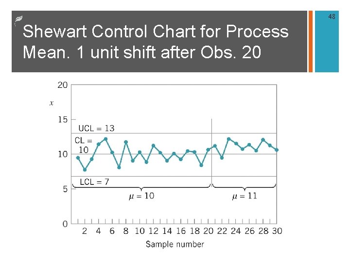
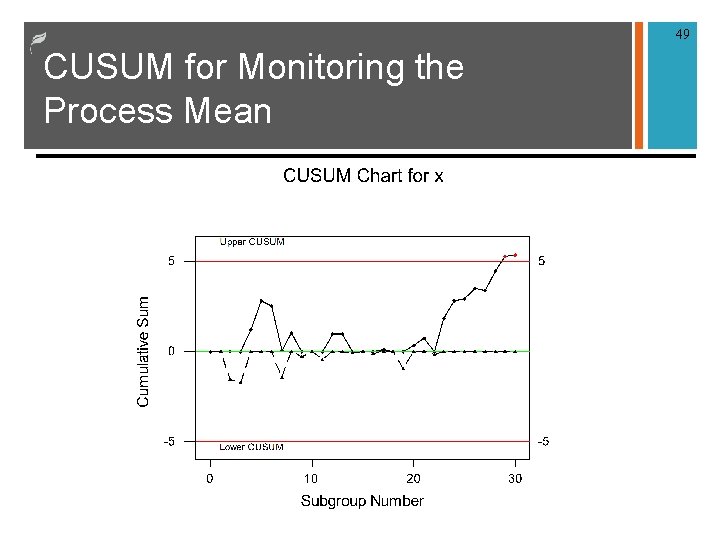
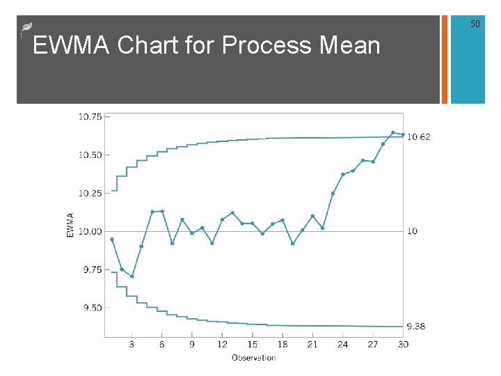
47 Use CUSUM or EWMA charts to detect small shifts faster n A third chart can be added to the traditional x-bar and R- charts for protecting against small shifts in the process mean (1 to 1. 5 standard deviations or less). These charts detect a small shift in half the number of points of traditional Shewart charts. Patterns are not useful because data points are correlated. n Cumulative Sum Chart (CUSUM) – It tracks the cumulative sum of the distance from the mean n Exponentially Weighted Moving Average (EWMA) – Uses exponential weighting to predict the next point.

48 Shewart Control Chart for Process Mean. 1 unit shift after Obs. 20

49 CUSUM for Monitoring the Process Mean

50 EWMA Chart for Process Mean

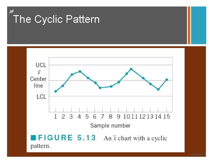
51 Failing to Detect Non-normal Patterns - 1 n Some assignable causes result in non-normal patterns that are not easily detected with traditional decision rules. Analogy would be EEG or EKG where trained eye can see patterns that reflect a health problem. n Cycles, trends – changing operators, changing shifts, tool or equipment wear, or temperature or humidity swings, can cause defects over time but go unrecognized on the control charts. n Hugging limits or centerline – Broken measurement equipment or operators fudging data can cause this.

The Cyclic Pattern 52 Chapter 5

53 Failing to Detect Non-normal Patterns - 2 n Recommendations n Training on how to recognize patterns n Some sort of historical data base to help people recognize patterns that repeat themselves. n Use of Six Sigma Black Belts to watch how control charts are being used. They can help recognize patterns and train operators.

54 Dealing with Low-Defect Levels n When defect levels or count rates in a process become very low, say under 1000 occurrences per million, then there are long periods of time between the occurrence of a nonconforming unit. n Zero defects occur n Control charts (u and c) with statistics consistently plotting at zero are uninformative. Introduction to Statistical Quality Control,

55 Dealing with Low-Defect Levels Alternative n Chart the time between successive occurrences of the counts – or time between events control charts. n If defects or counts occur according to a Poisson distribution, then the time between counts occur according to an exponential distribution. Introduction to Statistical Quality Control,

56 Dealing with Low-Defect Levels Consideration n Exponential distribution is skewed. n Corresponding control chart very asymmetric. n One possible solution is to transform the exponential random variable to a Weibull random variable using x = y 1/3. 6 (where y is an exponential random variable) – this Weibull distribution is well-approximated by a normal. n Construct a control chart on x assuming that x follows a normal distribution Introduction to Statistical Quality Control,

Choice Between Attributes and Variables Control Charts 57 n Each has its own advantages and disadvantages n Attributes data is easy to collect and several characteristics may be collected per unit. n Variables data can be more informative since information about the process mean and variance is obtained directly. n Variables control charts can indicate impending trouble and action may be taken before defectives are produced. n Attributes control charts will not react unless the process has already changed. Introduction to Statistical Quality Control,

58 Managing SPC n Black Belt or Master Black Belt should be able to set up the proper SPC Charts and monitor them. n Issues to address when designing SPC charts: n Proper type of chart to use for the situation n Decision rules being used n Is the process capable or not capable n Sample size and sample frequency n Sampling method n How assignable causes will be resolved n Continous training on how to interpret/use results