The Implicit Function TheoremPart 1 Equations in two

The Implicit Function Theorem---Part 1 Equations in two variables

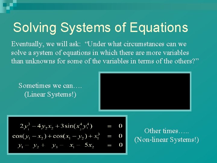
Solving Systems of Equations Eventually, we will ask: “Under what circumstances can we solve a system of equations in which there are more variables than unknowns for some of the variables in terms of the others? ” Sometimes we can…. (Linear Systems!) Other times…. . (Non-linear Systems!)

“Solving” Systems of Equations The existence of a “nice” solution vs Actually finding a solution

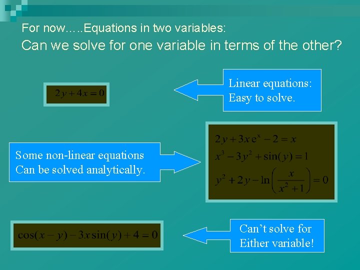
For now…. . Equations in two variables: Can we solve for one variable in terms of the other? Linear equations: Easy to solve. Some non-linear equations Can be solved analytically. Can’t solve for Either variable!

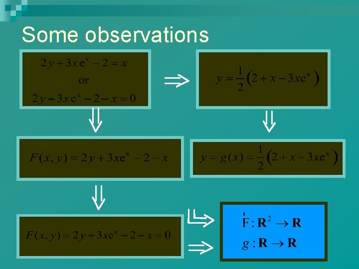
Some observations

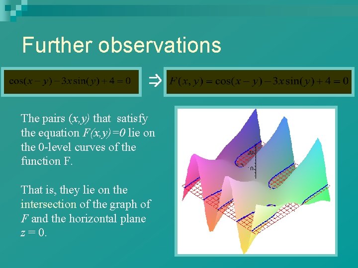
Further observations The pairs (x, y) that satisfy the equation F(x, y)=0 lie on the 0 -level curves of the function F. That is, they lie on the intersection of the graph of F and the horizontal plane z = 0.

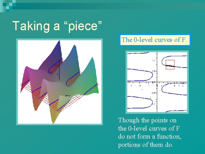
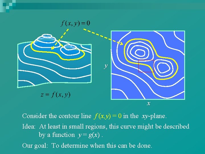
Taking a “piece” The 0 -level curves of F. Though the points on the 0 -level curves of F do not form a function, portions of them do.

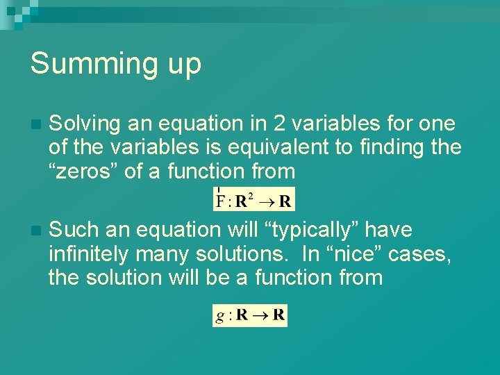
Summing up n Solving an equation in 2 variables for one of the variables is equivalent to finding the “zeros” of a function from n Such an equation will “typically” have infinitely many solutions. In “nice” cases, the solution will be a function from

More observations The previous diagrams show that, in general, the 0 -level curves are not the graph of a function. n But, even so, portions of them may be. n Indeed, if the function F is “well-behaved, ” we can hope to find a solution function in the neighborhood of a single known solution. n Well-behaved in this case means differentiable (locally planar). n

y x Consider the contour line f (x, y) = 0 in the xy-plane. Idea: At least in small regions, this curve might be described by a function y = g(x). Our goal: To determine when this can be done.

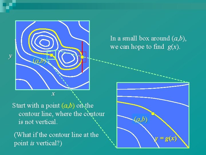
In a small box around (a, b), we can hope to find g(x). y (a, b) x Start with a point (a, b) on the contour line, where the contour is not vertical. (What if the contour line at the point is vertical? ) (a, b) y = g(x)

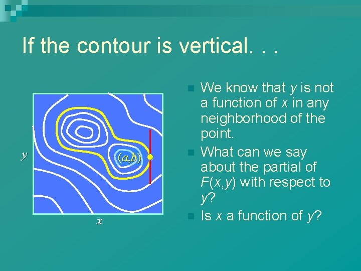
If the contour is vertical. . . n y (a, b) x n n We know that y is not a function of x in any neighborhood of the point. What can we say about the partial of F(x, y) with respect to y? Is x a function of y?

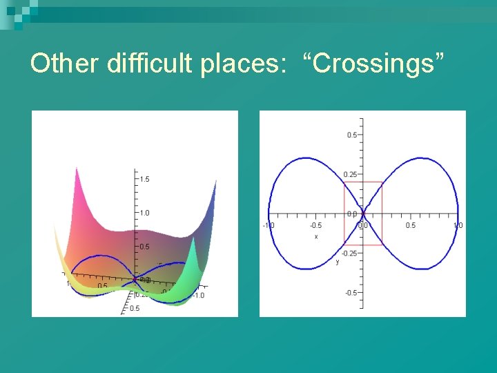
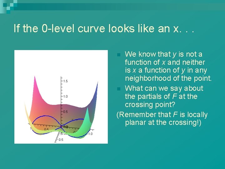
Other difficult places: “Crossings”

If the 0 -level curve looks like an x. . . We know that y is not a function of x and neither is x a function of y in any neighborhood of the point. n What can we say about the partials of F at the crossing point? (Remember that F is locally planar at the crossing!) n