The Impact of Overfitting and Overgeneralization on the

The Impact of Overfitting and Overgeneralization on the Classification Accuracy in Data Mining by Huy Nguyen Anh Pham and Evangelos Triantaphyllou INFORMS’ 2007 – Seattle, WA, November 4 - 7, 2007 Department of Computer Science, Louisiana State University Baton Rouge, LA 70803 Emails: hpham 15@lsu. edu and trianta@csc. lsu. edu 9/17/2021 1

Outline n n n n Motivation Problem definition Current work Some key observations The proposed methodology Rationale for the proposed methodology Some computational results Conclusions 9/17/2021 2

Motivation n The typical of a classification problem: q q q 9/17/2021 Given is a collection of records comprising the training set: n Each record contains a set of attributes and the corresponding class value. Find a classification model that describes each class as a function of the attributes. Use this model to classify new records of unknown class value. 3

Motivation – Cont’d n Some classification algorithms: q Decision Trees (DTs) [Quinlan, 1993]. q K-Nearest Neighbor Classifiers [Cover, 1995]. q Rule-based Classifiers [Cohen, 1995], [Clark, 1991]. q Bayes Classifiers [Langley, 1992], [Lewis, 1998]. q Artificial Neural Networks (ANNs) [Hecht-Nielsen, 1989] and [Abdi, 2003]. q Logic-based methods [Hammer and Boros, 1994], [Triantaphyllou, 1994]. q 9/17/2021 Support Vector Machines (SVMs) [Vapnik, 1979; and 1998] and [Cristianini and John, 2003]. 4

Motivation – Cont’d n Drawbacks of classification algorithms: q q 9/17/2021 DTs have been successful in the medical domain [Avrsnik J et. al. , 1995]. However, DTs have had some certain limitations when used in this domain [Kokol et. al. , 1998] and [Podgorelec, 2002]. SVMs have shown to be successful in bioinformatics, such as in [Byvatov, 2003] and [Huzefa et. al. , 2005]. At the same time, SVMs also did poorly in this field [Spizer et. al. , 2006]. Their performance is often times coincidental. Overfitting and overgeneralization problems may be the cause of this poor performance. 5

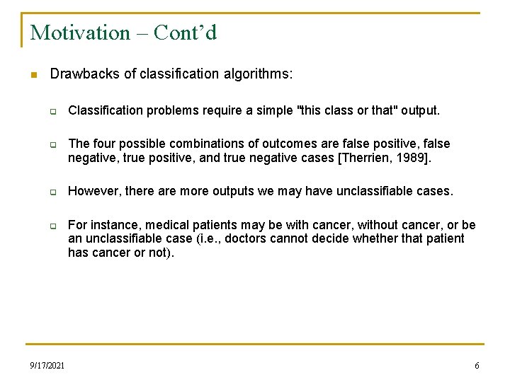
Motivation – Cont’d n Drawbacks of classification algorithms: q q 9/17/2021 Classification problems require a simple "this class or that" output. The four possible combinations of outcomes are false positive, false negative, true positive, and true negative cases [Therrien, 1989]. However, there are more outputs we may have unclassifiable cases. For instance, medical patients may be with cancer, without cancer, or be an unclassifiable case (i. e. , doctors cannot decide whether that patient has cancer or not). 6

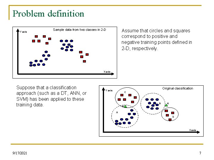
Problem definition Y axis Sample data from two classes in 2 -D Assume that circles and squares correspond to positive and negative training points defined in 2 -D, respectively. X axis Suppose that a classification approach (such as a DT, ANN, or SVM) has been applied to these training data. Original classification Y axis C B N M A D X axis 9/17/2021 7

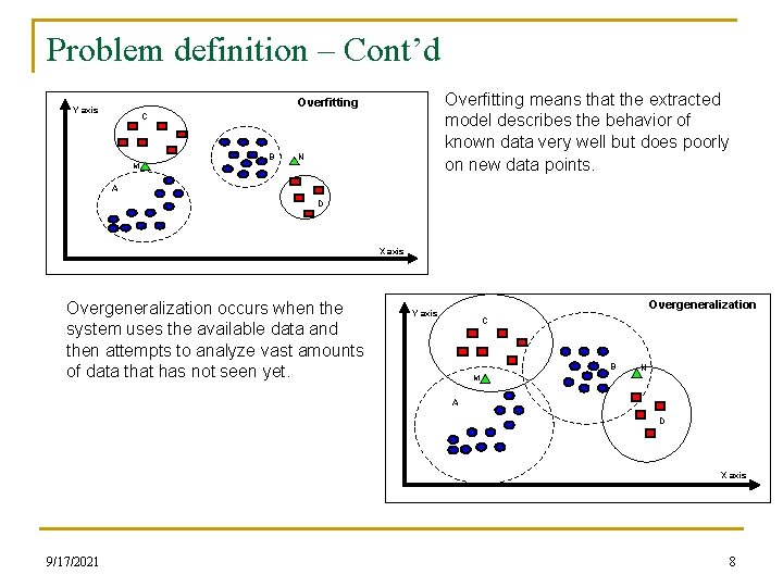
Problem definition – Cont’d Overfitting means that the extracted model describes the behavior of known data very well but does poorly on new data points. Overfitting Y axis C B N M A D X axis Overgeneralization occurs when the system uses the available data and then attempts to analyze vast amounts of data that has not seen yet. Overgeneralization Y axis C B N M A D X axis 9/17/2021 8

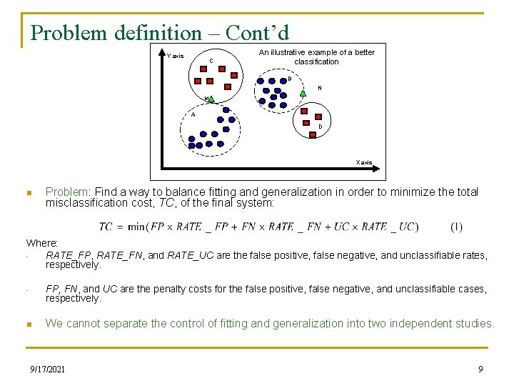
Problem definition – Cont’d Y axis C An illustrative example of a better classification B N M A D X axis n Problem: Find a way to balance fitting and generalization in order to minimize the total misclassification cost, TC, of the final system: Where: RATE_FP, RATE_FN, and RATE_UC are the false positive, false negative, and unclassifiable rates, respectively. - FP, FN, and UC are the penalty costs for the false positive, false negative, and unclassifiable cases, respectively. n We cannot separate the control of fitting and generalization into two independent studies. 9/17/2021 9

Outline n n n n Motivation Problem definition Current work Some key observations The proposed methodology Rationale for the proposed methodology Some computational results Conclusions 9/17/2021 10

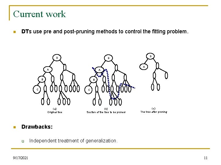
Current work n DTs use pre and post-pruning methods to control the fitting problem. D A A A B B C C (a) Original tree n D D (b) Section of the tree to be pruned (c) The tree after pruning Drawbacks: q 9/17/2021 Independent treatment of generalization. 11

Current work – Cont’d n Rule-based Classifiers q q n Use two strategies for growing the classification rules: general-to-specific and specific-to-general. Then, use rule pruning methods to decrease their generalization errors. Drawbacks: q The complexity for finding optimal rules is of exponential size of the search space. q Independent treatment of generalization. 9/17/2021 12

Current work – Cont’d K-Nearest Neighbor Classifiers find K training points that are relatively similar to attributes of a testing point to determine the class label. n A wrong value for K may lead to the overfitting or the overgeneralization problems. q The value for K can be chosen by a distance-weighted voting scheme [Dudani, 1976] and [Keller, Gray and Givens, 1985]. q Drawbacks: n q Classifying a test point can be quite expensive. q It may be unstable since it is based on local information. q 9/17/2021 It is difficult to find an appropriate value for K in order to avoid overfitting and overgeneralization. 13

Current work – Cont’d n Bayes Classifiers use modeling probabilistic relationships between the attributes and the class value for solving classification problems: q q n Naïve Bayes (NBs) assume that all the attributes are independent. Bayesian Belief Networks (BBNs) allow for pairs of attributes which can be conditionally independent. Drawbacks: q q 9/17/2021 NBs and BBNs may suffer of overfitting because they combine probabilistically the data with prior knowledge. Independent treatment of fitting. 14

Current work – Cont’d n n Artificial Neural Networks (ANNs) determine a set of weights in order to minimize the total sum of misclassification cost. q The network topology depends on both the number of the weights and their sizes. q The network topology may lead to overfitting or overgeneralization problems. Drawbacks: q q 9/17/2021 It is difficult to find an appropriate network topology for a given problem in order to avoid overfitting or overgeneralization. It may take lots of time for training an ANN when the number of hidden nodes is large. 15

Current work – Cont’d n n Support Vector Machines (SVMs) find maximal margin hyperplanes which separate training points. q Decision boundaries with maximal margins tend to lead to better generalization. q SVMs attempt to formulate the learning problem as a convex optimization problem. Drawbacks: q q 9/17/2021 Independent treatment of generalization. Formulating the learning problem as a convex optimization problem may lead to overgeneralization because it may be the cause of too many misclassifications. 16

Outline n n n n Motivation Problem definition Current work Some key observations The proposed methodology Rationale for the proposed methodology Some computational results Conclusions 9/17/2021 17

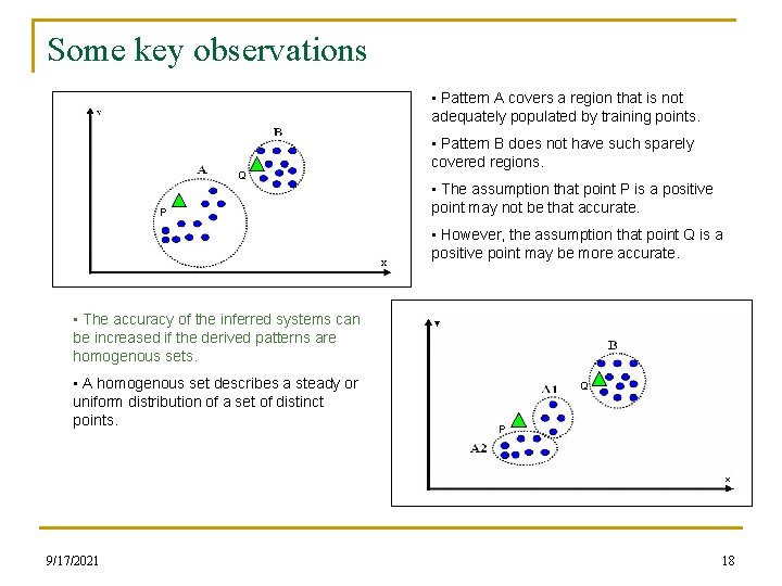
Some key observations • Pattern A covers a region that is not adequately populated by training points. Q P • Pattern B does not have such sparely covered regions. • The assumption that point P is a positive point may not be that accurate. • However, the assumption that point Q is a positive point may be more accurate. • The accuracy of the inferred systems can be increased if the derived patterns are homogenous sets. • A homogenous set describes a steady or uniform distribution of a set of distinct points. 9/17/2021 Q P 18

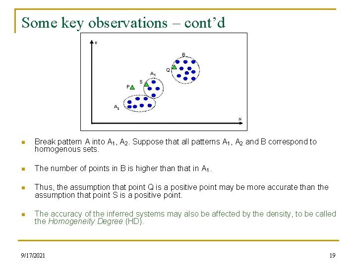
Some key observations – cont’d B A 1 P Q S A 2 n Break pattern A into A 1, A 2. Suppose that all patterns A 1, A 2 and B correspond to homogenous sets. n The number of points in B is higher than that in A 1. n Thus, the assumption that point Q is a positive point may be more accurate than the assumption that point S is a positive point. n The accuracy of the inferred systems may also be affected by the density, to be called the Homogeneity Degree (HD). 9/17/2021 19

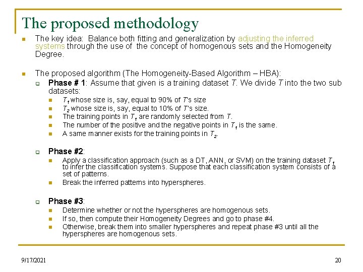
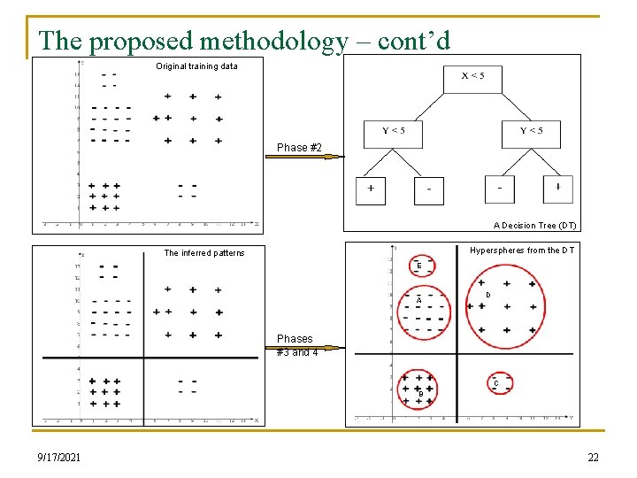
The proposed methodology n The key idea: Balance both fitting and generalization by adjusting the inferred systems through the use of the concept of homogenous sets and the Homogeneity Degree. n The proposed algorithm (The Homogeneity-Based Algorithm – HBA): q Phase # 1: Assume that given is a training dataset T. We divide T into the two sub datasets: n n n q Phase #2: n n q Apply a classification approach (such as a DT, ANN, or SVM) on the training dataset T 1 to infer the classification systems. Suppose that each classification system consists of a set of patterns. Break the inferred patterns into hyperspheres. Phase #3: n n n 9/17/2021 T 1 whose size is, say, equal to 90% of T’s size T 2 whose size is, say, equal to 10% of T’s size. The training points in T 1 are randomly selected from T. The number of the positive and the negative points in T 1 is the same. A same manner exists for the training points in T 2. Determine whether or not the hyperspheres are homogenous sets. If so, then compute their Homogeneity Degrees and go to phase #4. Otherwise, break them into smaller hyperspheres and repeat phase #3 until all the hyperspheres are homogenous sets. 20

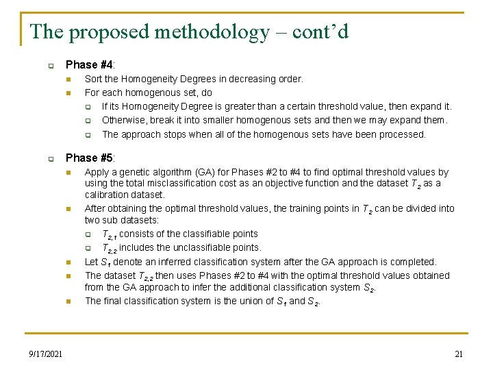
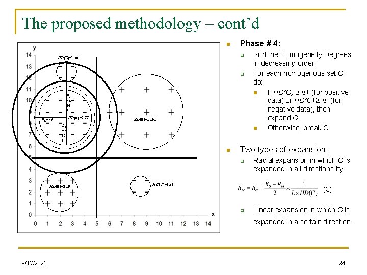
The proposed methodology – cont’d q Phase #4: n n q Phase #5: n n n 9/17/2021 Sort the Homogeneity Degrees in decreasing order. For each homogenous set, do q If its Homogeneity Degree is greater than a certain threshold value, then expand it. q Otherwise, break it into smaller homogenous sets and then we may expand them. q The approach stops when all of the homogenous sets have been processed. Apply a genetic algorithm (GA) for Phases #2 to #4 to find optimal threshold values by using the total misclassification cost as an objective function and the dataset T 2 as a calibration dataset. After obtaining the optimal threshold values, the training points in T 2 can be divided into two sub datasets: q T 2, 1 consists of the classifiable points q T 2, 2 includes the unclassifiable points. Let S 1 denote an inferred classification system after the GA approach is completed. The dataset T 2, 2 then uses Phases #2 to #4 with the optimal threshold values obtained from the GA approach to infer the additional classification system S 2. The final classification system is the union of S 1 and S 2. 21

The proposed methodology – cont’d Original training data Phase #2 A Decision Tree (DT) Hyperspheres from the DT The inferred patterns E A D Phases #3 and 4 C B 9/17/2021 22

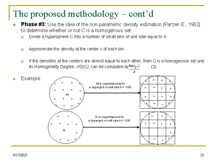
The proposed methodology – cont’d n Phase #3: Use the idea of the non-parametric density estimation [Parzen E. , 1962] to determine whether or not C is a homogenous set: q Divide a hypersphere C into a number of small bins of unit side equal to h. q Approximate the density at the center x of each bin. q n If the densities at the centers are almost equal to each other, then C is a homogenous set and its Homogeneity Degree, HD(C), can be computed by (2). Example: + + + + M is superimposed to a hypergrid of unit size h = 1. 00. M + + + N + 9/17/2021 + + + + + N is superimposed to a hypergrid of unit size h = 1. 00. + + + + 23

The proposed methodology – cont’d n Phase # 4: q HD(E)=1. 38 q RC =4. 24 2 HD(A)=2. 77 RM=2. 5 HD(D)=1. 151 RA =2. 12 1 n Two types of expansion: q HD(B)=2. 19 Sort the Homogeneity Degrees in decreasing order. For each homogenous set C, do: n If HD(C) ≥ β+ (for positive data) or HD(C) ≥ β- (for negative data), then expand C. n Otherwise, break C. HD(C)=1. 38 Radial expansion in which C is expanded in all directions by: (3). q Linear expansion in which C is expanded in a certain direction. 9/17/2021 24

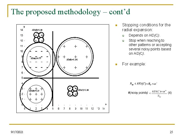
The proposed methodology – cont’d n HD(E)=1. 38 Stopping conditions for the radial expansion: q q HD(A)=2. 77 HD(D)=1. 151 n HD(B)=2. 19 9/17/2021 Depends on HD(C). Stop when reaching to other patterns or accepting several noisy points based on HD(C)=1. 38 For example: #(noisy points) (4) 25

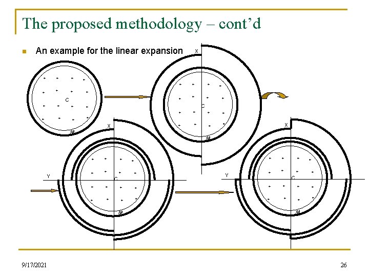
The proposed methodology – cont’d n An example for the linear expansion + + + + + + C + X C + + + + + X X M M Y + + + + C + + + + M 9/17/2021 + M 26

Outline n n n n Motivation Problem definition Current work Some key observations The proposed methodology Rationale for the proposed methodology Some computational results Conclusions 9/17/2021 27

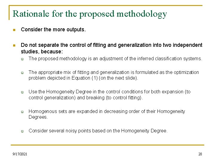
Rationale for the proposed methodology n Consider the more outputs. n Do not separate the control of fitting and generalization into two independent studies, because: q q q 9/17/2021 The proposed methodology is an adjustment of the inferred classification systems. The appropriate mix of fitting and generalization is formulated as the optimization problem depicted in Equation (1) (on the next slide). Use the Homogeneity Degree in the control conditions for both expansion (to control generalization) and breaking (to control fitting). Homogenous sets are expanded in decreasing order of their Homogeneity Degrees. Consider several noisy points based on the Homogeneity Degree. 28

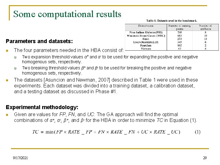
Some computational results Parameters and datasets: n The four parameters needed in the HBA consist of: q q n Two expansion threshold values α+ and α- to be used for expanding the positive and negative homogenous sets, respectively. Two breaking threshold values β+ and β- to be used for breaking the positive and negative homogenous sets, respectively. The datasets [Asuncion and Newman, 2007] described in Table 1 were used in these experiments. Each dataset was divided into a training dataset, a calibration dataset, and a testing dataset as discussed in Phase #1. Experimental methodology: n Given are values for FP, FN, and UC. The GA approach will find the optimal combinations of α+, α-, β+, and β- for the HBA in order to minimize TC in Equation (1). 9/17/2021 29

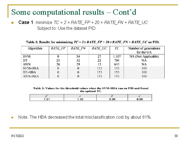
Some computational results – Cont’d n Case 1: minimize TC = 2 × RATE_FP + 20 × RATE_FN + RATE_UC Subject to: Use the dataset PID n Note: The HBA decreased the total misclassification cost by about 81%. 9/17/2021 30

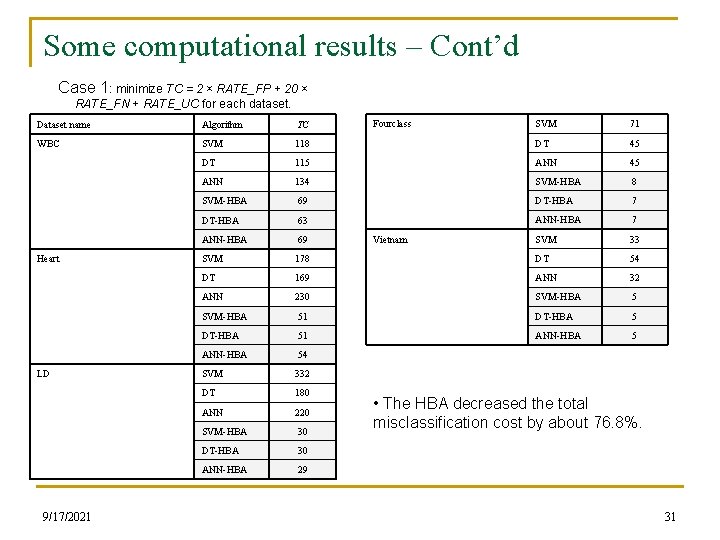
Some computational results – Cont’d Case 1: minimize TC = 2 × RATE_FP + 20 × RATE_FN + RATE_UC for each dataset. SVM 71 118 DT 45 DT 115 ANN 45 ANN 134 SVM-HBA 8 SVM-HBA 69 DT-HBA 7 DT-HBA 63 ANN-HBA 7 ANN-HBA 69 SVM 33 SVM 178 DT 54 DT 169 ANN 32 ANN 230 SVM-HBA 51 DT-HBA 51 ANN-HBA 54 SVM 332 DT 180 ANN 220 SVM-HBA 30 DT-HBA 30 ANN-HBA 29 Dataset name Algorithm TC WBC SVM Heart LD 9/17/2021 Fourclass Vietnam • The HBA decreased the total misclassification cost by about 76. 8%. 31

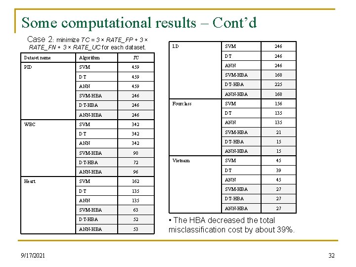
Some computational results – Cont’d Case 2: minimize TC = 3 × RATE_FP + 3 × RATE_FN + 3 × RATE_UC for each dataset. LD SVM 246 Dataset name Algorithm TC DT 246 PID SVM 459 ANN 246 DT 459 SVM-HBA 168 ANN 459 DT-HBA 225 SVM-HBA 246 ANN-HBA 168 DT-HBA 246 SVM 156 ANN-HBA 246 DT 135 SVM 342 ANN 135 DT 342 SVM-HBA 21 ANN 342 DT-HBA 15 SVM-HBA 90 ANN-HBA 15 DT-HBA 72 SVM 45 ANN-HBA 96 DT 39 SVM 162 ANN 45 DT 135 SVM-HBA 27 ANN 135 DT-HBA 27 SVM-HBA 63 ANN-HBA 27 DT-HBA 52 ANN-HBA 53 WBC Heart 9/17/2021 Fourclass Vietnam • The HBA decreased the total misclassification cost by about 39%. 32

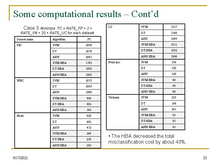
Some computational results – Cont’d Case 3: Minimize TC = RATE_FP + 2 × RATE_FN + 20 × RATE_UC for each dataset. LD 1357 DT 1168 ANN 1094 Dataset name Algorithm PID SVM 2034 SVM-HBA 1011 DT 2074 DT-HBA 1032 ANN 2041 ANN-HBA 1086 SVM-HBA 1763 SVM 138 DT-HBA 1803 DT 120 ANN-HBA 1803 ANN 120 SVM 2073 SVM-HBA 46 DT 2043 DT-HBA 46 ANN 1990 ANN-HBA 66 SVM-HBA 486 SVM 223 DT-HBA 602 DT 168 ANN-HBA 542 ANN 241 SVM 624 SVM-HBA 85 DT 602 DT-HBA 85 ANN 472 ANN-HBA 85 SVM-HBA 268 DT-HBA 258 ANN-HBA 202 WBC Heart 9/17/2021 TC SVM Fourclass Vietnam • The HBA decreased the total misclassification cost by about 43%. 33

Conclusions n We identified a gap between fitting and generalization in current algorithms. n Defined the goal as an optimization problem. n Provided a new approach which appears to be very promising. Thank you Any questions? 9/17/2021 34