The Impact of Lateral Boundary Conditions on CMAQ

The Impact of Lateral Boundary Conditions on CMAQ Predictions over the Continental US: a Sensitivity Study Compared to Ozonsonde Data Youhua Tang*, Pius Lee, Marina Tsidulko, Ho-Chun Huang, Scientific Applications International Corporation, Camp Springs, Maryland Jeffery T. Mc. Queen, Geoffrey J. Di. Mego NOAA/NWS/National Centers for Environmental Prediction, Camp Springs, Maryland. Louisa K. Emmons National Center for Atmospheric Research, Boulder, Colorado Robert B. Pierce NOAA/NESDIS Advanced Satellite Products Branch, Madison, Wisconsin Hsin-Mu Lin, Daiwen Kang, Daniel Tong, Shao-cai Yu Science and Technology Corporation, Hampton, VA. Rohit Mathur, Jonathan E. Pleim, Tanya L. Otte, George Pouliot, Jeffrey O. Young, Kenneth L. Schere NOAA-OAR/ARL, Research Triangle Park, NC. (On assignment to the National Exposure Research Laboratory, U. S. E. P. A. ) and Paula M. Davidson Office of Science and Technology, NOAA/National Weather Service, Silver Spring, MD

Objective • Current operational CMAQ forecast over continental USA uses static lateral boundary condition as the external influences from transport outside the CMAQ domain are relatively weak compared to emissions within the model domain. • Here we try to use sensitivity study to assess the impact of using lateral boundary conditions from global models during typical summertime ozone episode compared to IONS (INTEX Ozone-sonde Network Study) ozonesonde and EPA airnow data.

WRF-NMM/CMAQ Model Configuration • Driven by hourly meteorological forecasts from the operational North America Mesoscale (NAM) WRF-NMM prediction system. • The operational CMAQ system covering Continental USA in 12 km horizontal resolution Carbon Bond Mechanism-4 (CBM 4) 22 vertical layers up to 100 h. Pa. vertical diffusivity and dry deposition based on Pleim and Xu (2001), scale J-table for photolysis attenuation due to cloud Asymmeric Convective Scheme (ACM) (Pleim and Chang, 1992).

Global Models as CMAQ LBC Providers MOZART RAQMS GFS O 3 Horizontal Resolution 2. 8 2 2 0. 31 Meteorology GFS analysis GFS forecasts Anthropogenic emissions Granier et al. , 2004 GEIA/EDGAR inventory with updated Asian emission (Streets et al. 2003) Not applicable Biomass burning emissions GFED-v 2 (van der Werf, 2006) ecosystem/severity based Not applicable stratospheric ozone synthetic ozone constraint (Mc. Linden et al. , 2000) OMI/TES assimilation (Pierce et al. , 2007) Initialized by SBUV-2 Input frequency to CMAQ Every 3 hours Every 6 hours hourly

VOC Species mapping tables between RAQMS/MOZART species and CMAQ CBM-IV (other species in the same names are converted directly) RAQMS Species CH 3 OOH (Methyl hydroperoxide) CMAQ CBM-IV UMHP C 2 H 6 2* PAR OLET (terminal alkenes) OLE 1+PAR OLEI (internal alkenes) OLE 2 + 2*PAR MOZART Species CMAQ CBM-IV CH 3 OOH (Methyl UMHP hydroperoxide) CH 3 CHO ALD 2 C 2 H 6 2*PAR C 3 H 8 3*PAR BIGALK (higher alkanes) 4*PAR C 3 H 6 OLE + 2*PAR BIGENE (higher alkenes) OLE + 3*PAR C 10 H 16 (terpene) OLE + 9*PAR

Fixed LBC MOZART High vertical variability RAQMS GFS O 3 Strong gradient near marine boundary layer

Another method is using mean ozonesonde profiles as boundary condition

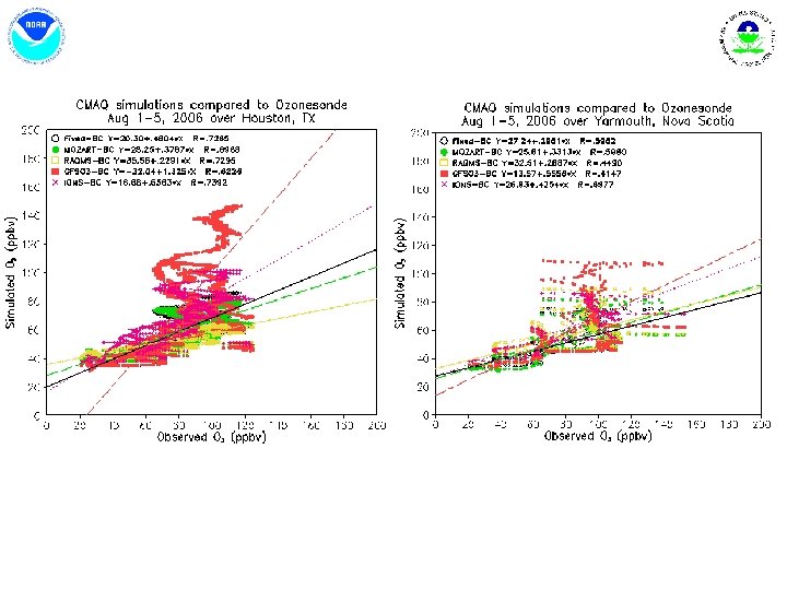
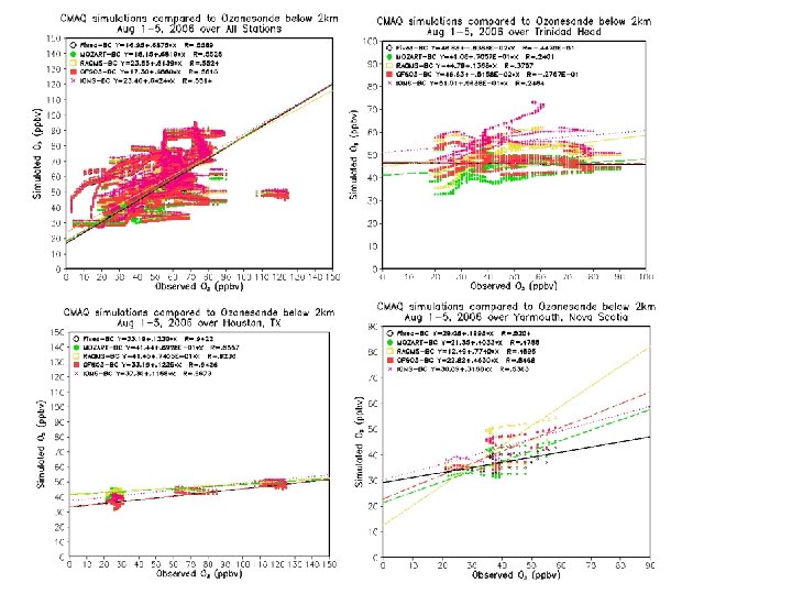
Model predictions using different LBCs compared to IONS ozonesonde

Other O 3 LBCs have higher O 3 in the upper layers than the original Fixed BC over most areas

Global models MOZART and RAQMS show better correlations over all stations and west coast that faces major inflows.

Mean O 3 Difference (ppbv) (MOZAT-BC – Fixed-BC) Fixed-BC Predicted Mean O 3 (ppbv) Mean O 3 bias (ppbv) Compared to EPA Airnow data

RAQMS GFS O 3 IONS Mean O 3 bias (ppbv) Compared to EPA Airnow data

CMAQ simulations compared to AIRNOW hourly O 3 data from Aug 1 to 5 All AIRNOW Stations West of -115 W North of 43 N Fixed BC S=0. 887 R=0. 714 MB=8. 0 ppbv S=0. 804 R=0. 691 MB=4. 7 ppbv S=0. 873 R=0. 737 MB=7. 5 ppbv RAQMS BC S=0. 911 R=0. 718 MB=10. 0 ppbv S=0. 914 R=0. 703 MB=7. 1 ppbv S=0. 942 R=0. 742 MB=10. 0 ppbv MOZART BC S=0. 941 R=0. 716 MB=8. 2 ppbv S=0. 872 R=0. 730 MB=2. 2 ppbv S=0. 985 R=0. 743 MB=6. 9 ppbv GFS O 3 BC S=0. 935 R=0. 714 MB=9. 2 ppbv S=0. 820 R=0. 697 MB=4. 8 ppbv S=0. 922 R=0. 724 MB=9. 0 ppbv IONS BC S=0. 923 R=0. 719 MB=11. 1 ppbv S=0. 883 R=0. 680 MB=10. 8 ppbv S=0. 871 R=0. 712 MB=11. 4 ppbv S is correlation slope, R is correlation coefficient, and MB is mean bias

Summary • During this scenario, the impact of lateral boundary condition is remarkable. The model predictions using different LBC show different performances varied from location to location. • Full-chemistry MOZART and RAQMS LBC have the stronger impact on surface ozone prediction that of GFS-O 3. • Using observed IONS ozonesonde as LBC could work over some locations, but it tends to overpredict surface ozone due to its relatively coarse spatial and temporal resolutions. How the model properly handle the observed profiles is also an issue.

Acknowledgements: We thank Dr. Anne Thompson for INTEX Ozone-sonde Network Study (IONS) ozonesonde data, and EPA for providing AIRNOW data.