The Human Population Growth and Distribution G Tyler
The Human Population: Growth and Distribution G. Tyler Miller, Jr. ’s Environmental Science 10 th Edition Chapter 11
Key Concepts Ø Factors affecting human population size Ø Human population problems Ø Managing population growth Ø Urban growth Ø Resource and environmental problems in urban areas Ø Transportation in urban areas Ø Achieving sustainable cities
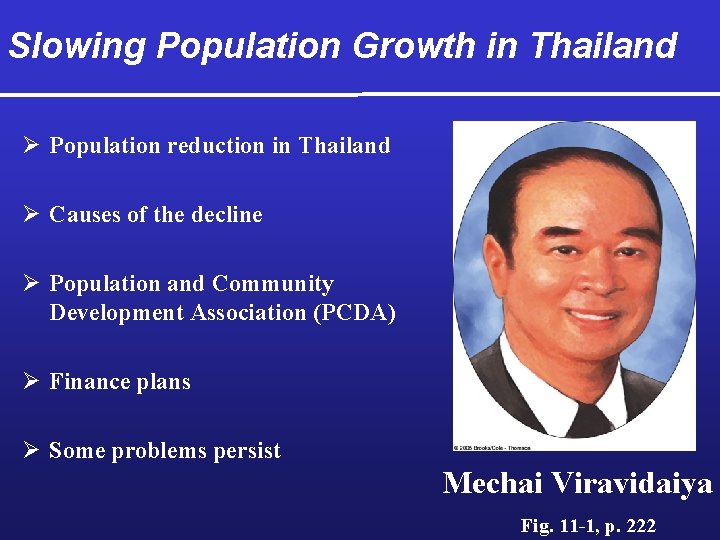
Slowing Population Growth in Thailand Ø Population reduction in Thailand Ø Causes of the decline Ø Population and Community Development Association (PCDA) Ø Finance plans Ø Some problems persist Mechai Viravidaiya Fig. 11 -1, p. 222
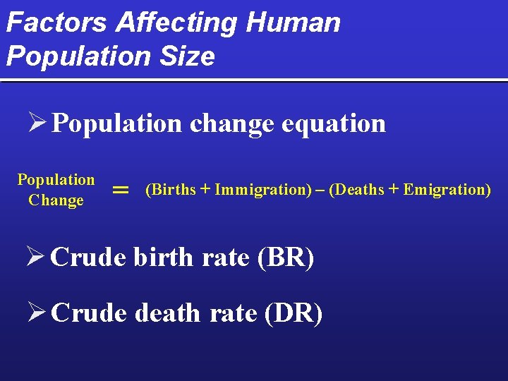
Factors Affecting Human Population Size Ø Population change equation Population Change = (Births + Immigration) – (Deaths + Emigration) Ø Crude birth rate (BR) Ø Crude death rate (DR)
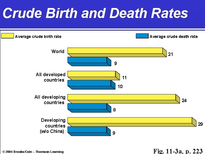
Crude Birth and Death Rates Average crude birth rate Average crude death rate World 21 9 All developed countries 11 10 All developing countries 24 8 Developing countries (w/o China) © 2004 Brooks/Cole – Thomson Learning 29 9 Fig. 11 -3 a, p. 223
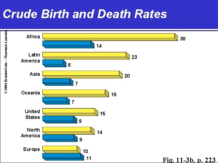
© 2004 Brooks/Cole – Thomson Learning Crude Birth and Death Rates Africa 38 14 Latin America 23 6 Asia 20 7 Oceania 18 7 United States North America Europe 15 9 14 9 10 11 Fig. 11 -3 b, p. 223
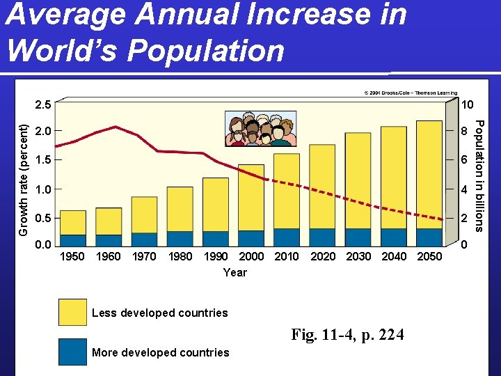
2. 5 10 2. 0 8 1. 5 6 1. 0 4 0. 5 2 0. 0 0 1950 1960 1970 1980 1990 2000 2010 Year 2020 2030 2040 2050 Less developed countries Fig. 11 -4, p. 224 More developed countries Population in billions Growth rate (percent) Average Annual Increase in World’s Population
Describing Population Changes ØReplacement-level fertility ØTotal fertility rate (TFR) ØWorld population projections ØUS fertility rates
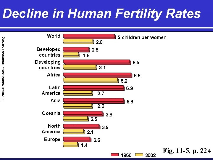
© 2004 Brooks/Cole – Thomson Learning Decline in Human Fertility Rates World 5 children per women 2. 8 Developed countries Developing countries Africa 2. 5 1. 6 6. 5 3. 1 5. 2 Latin America 5. 9 2. 7 Asia 5. 9 2. 6 Oceania 2. 5 North America 2. 1 Europe 1. 4 6. 6 3. 8 3. 5 2. 6 1950 2002 Fig. 11 -5, p. 224
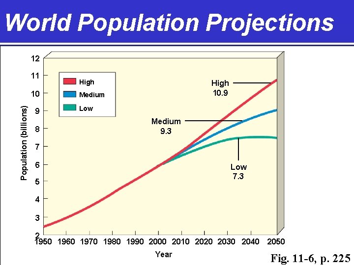
World Population Projections 12 11 Population (billions) 10 9 8 High 10. 9 Medium Low Medium 9. 3 7 6 Low 7. 3 5 4 3 2 1950 1960 1970 1980 1990 2000 2010 2020 2030 2040 Year 2050 Fig. 11 -6, p. 225
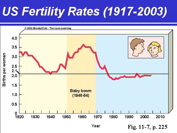
US Fertility Rates (1917 -2003) 4. 0 Births per woman 3. 5 3. 0 2. 5 2. 1 2. 0 1. 5 Baby boom (1946 -64) 1. 0 0. 5 0 1920 1930 1940 1950 1960 1970 Year 1980 1990 2000 2010 Fig. 11 -7, p. 225
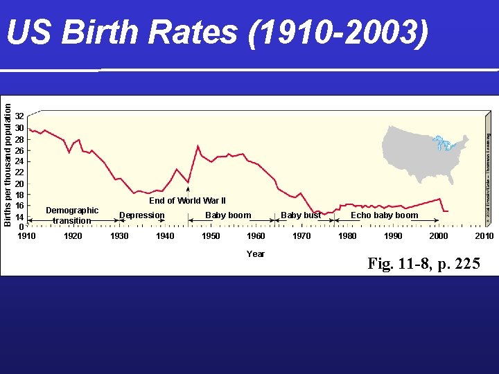
Births per thousand population US Birth Rates (1910 -2003) 32 30 28 26 24 22 20 18 16 14 0 1910 End of World War II Demographic transition 1920 Depression 1930 1940 Baby boom 1950 1960 Year Baby bust 1970 Echo baby boom 1980 1990 2000 2010 Fig. 11 -8, p. 225
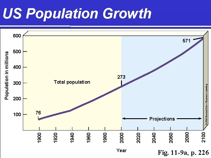
US Population Growth 571 500 400 273 Total population 300 200 76 Year 2100 2080 2060 2040 2020 2000 1980 1960 1940 Projections 1920 100 1900 Population in millions 600 Fig. 11 -9 a, p. 226
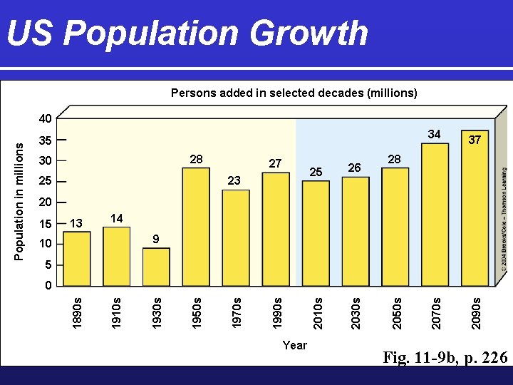
US Population Growth Persons added in selected decades (millions) 25 37 2090 s 23 26 34 2070 s 25 27 2030 s 28 30 2010 s 35 28 20 15 13 14 9 10 5 Year 2050 s 1990 s 1970 s 1950 s 1930 s 1910 s 0 1890 s Population in millions 40 Fig. 11 -9 b, p. 226
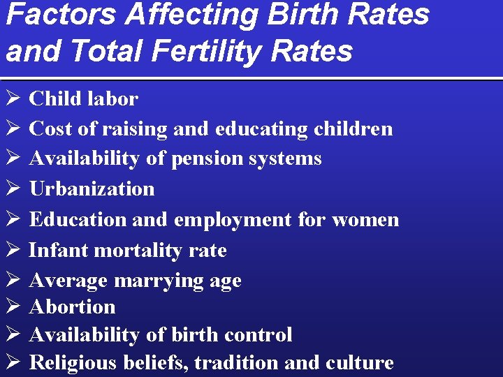
Factors Affecting Birth Rates and Total Fertility Rates Ø Child labor Ø Cost of raising and educating children Ø Availability of pension systems Ø Urbanization Ø Education and employment for women Ø Infant mortality rate Ø Average marrying age Ø Abortion Ø Availability of birth control Ø Religious beliefs, tradition and culture
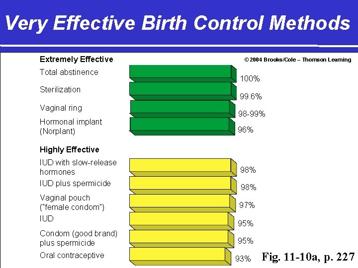
Very Effective Birth Control Methods Extremely Effective Total abstinence Sterilization Vaginal ring Hormonal implant (Norplant) © 2004 Brooks/Cole – Thomson Learning 100% 99. 6% 98 -99% 96% Highly Effective IUD with slow-release hormones IUD plus spermicide 98% Vaginal pouch (“female condom”) IUD 97% Condom (good brand) plus spermicide Oral contraceptive 98% 95% 93% Fig. 11 -10 a, p. 227
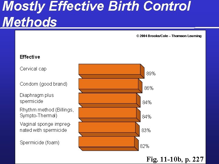
Mostly Effective Birth Control Methods © 2004 Brooks/Cole – Thomson Learning Effective Cervical cap Condom (good brand) 89% 86% Diaphragm plus spermicide 84% Rhythm method (Billings, Sympto-Thermal) 84% Vaginal sponge impregnated with spermicide 83% Spermicide (foam) 82% Fig. 11 -10 b, p. 227
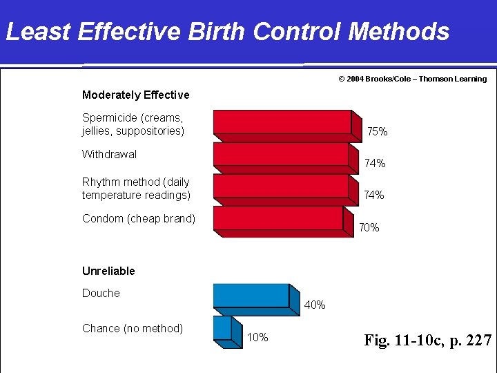
Least Effective Birth Control Methods © 2004 Brooks/Cole – Thomson Learning Moderately Effective Spermicide (creams, jellies, suppositories) 75% Withdrawal 74% Rhythm method (daily temperature readings) 74% Condom (cheap brand) 70% Unreliable Douche Chance (no method) 40% 10% Fig. 11 -10 c, p. 227
Factors Affecting Death Rates Ø Life expectancy Ø Infant mortality rate (IMR) Ø AIDS and other diseases
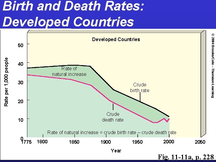
Birth and Death Rates: Developed Countries © 2004 Brooks/Cole – Thomson Learning Developed Countries Rate per 1, 000 people 50 40 Rate of natural increase 30 Crude birth rate 20 Crude death rate 10 Rate of natural increase = crude birth rate – crude death rate 0 1775 1800 1850 1900 Year 1950 2000 2050 Fig. 11 -11 a, p. 228
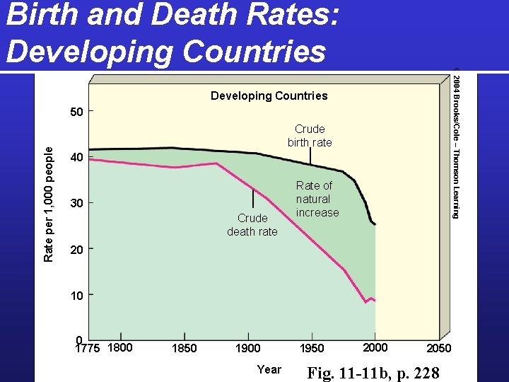
© 2004 Brooks/Cole – Thomson Learning Birth and Death Rates: Developing Countries Rate per 1, 000 people 50 Crude birth rate 40 30 Crude death rate Rate of natural increase 20 10 0 1775 1800 1850 1900 Year 1950 2000 2050 Fig. 11 -11 b, p. 228
Immigration into the US Ø Source of immigrants into the US Ø Arguments to reduce immigration Ø Arguments for immigration into the US
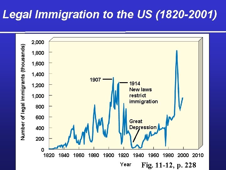
Number of legal immigrants (thousands) Legal Immigration to the US (1820 -2001) 2, 000 1, 800 1, 600 1, 400 1, 200 1, 000 800 600 400 1907 1914 New laws restrict immigration Great Depression 200 0 1820 1840 1860 1880 1900 1920 1940 1960 1980 2000 2010 Year Fig. 11 -12, p. 228
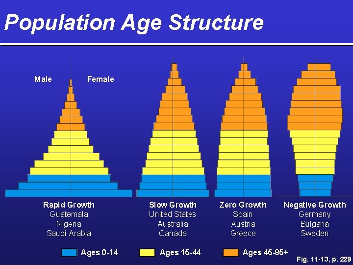
Population Age Structure Male Female Rapid Growth Guatemala Nigeria Saudi Arabia Ages 0 -14 Slow Growth United States Australia Canada Ages 15 -44 Zero Growth Spain Austria Greece Negative Growth Germany Bulgaria Sweden Ages 45 -85+ Fig. 11 -13, p. 229
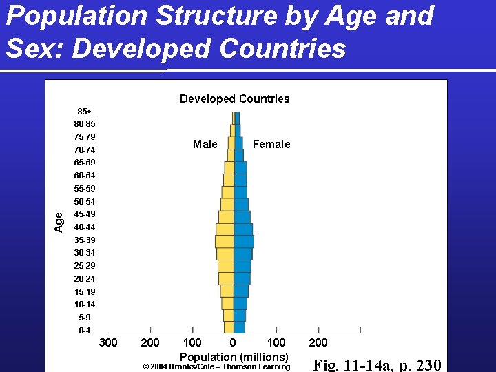
Population Structure by Age and Sex: Developed Countries 85+ 80 -85 75 -79 Male 70 -74 Female 65 -69 60 -64 55 -59 Age 50 -54 45 -49 40 -44 35 -39 30 -34 25 -29 20 -24 15 -19 10 -14 5 -9 0 -4 300 200 100 Population (millions) © 2004 Brooks/Cole – Thomson Learning 200 Fig. 11 -14 a, p. 230
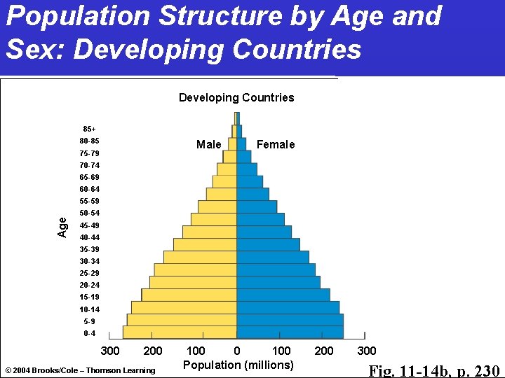
Population Structure by Age and Sex: Developing Countries 85+ 80 -85 Male 75 -79 Female 70 -74 65 -69 60 -64 Age 55 -59 50 -54 45 -49 40 -44 35 -39 30 -34 25 -29 20 -24 15 -19 10 -14 5 -9 0 -4 300 200 © 2004 Brooks/Cole – Thomson Learning 100 0 100 Population (millions) 200 300 Fig. 11 -14 b, p. 230
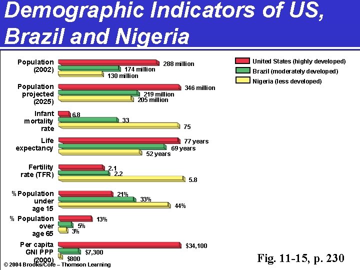
Demographic Indicators of US, Brazil and Nigeria Population (2002) 174 million 130 million Population projected (2025) Infant mortality rate 6. 8 33 Per capita GNI PPP (2000) 346 million 77 years 69 years 2. 1 2. 2 21% 5% 3% $800 Nigeria (less developed) 75 52 years Fertility rate (TFR) United States (highly developed) Brazil (moderately developed) 219 million 205 million Life expectancy %Population under age 15 % Population over age 65 288 million 5. 8 33% 44% 13% $7, 300 © 2004 Brooks/Cole – Thomson Learning $34, 100 Fig. 11 -15, p. 230
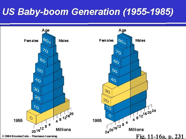
US Baby-boom Generation (1955 -1985) Age Females Males 1955 12 16 20 8 4 20 16 12 4 8 Millions © 2004 Brooks/Cole – Thomson Learning Females 1985 24 1612 20 Males 8 4 4 16 20 8 12 24 Millions Fig. 11 -16 a, p. 231
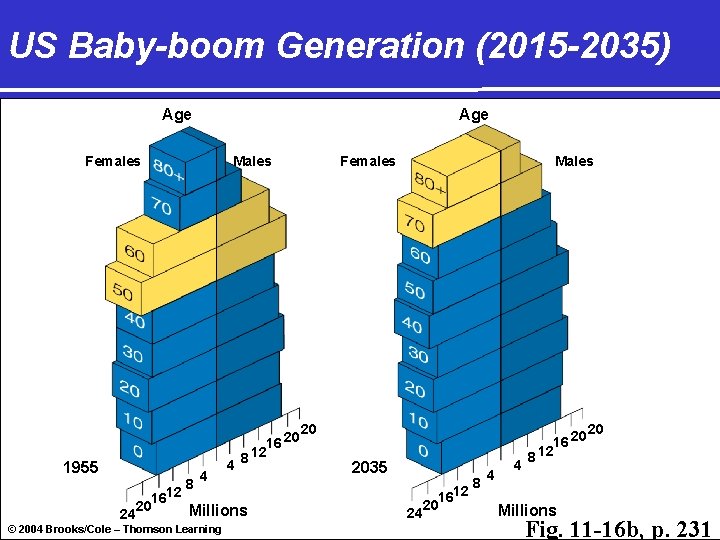
US Baby-boom Generation (2015 -2035) Age Females 1955 Males 4 4 16 20 8 12 8 1612 20 Millions 24 © 2004 Brooks/Cole – Thomson Learning Females Males 20 2035 24 1612 20 8 4 4 16 20 12 8 Millions 20 Fig. 11 -16 b, p. 231
Effects of Rapid Population Declines Ø 38 nations have stable populations Ø Rapid declines create social and economic problems Ø Labor and social security problems
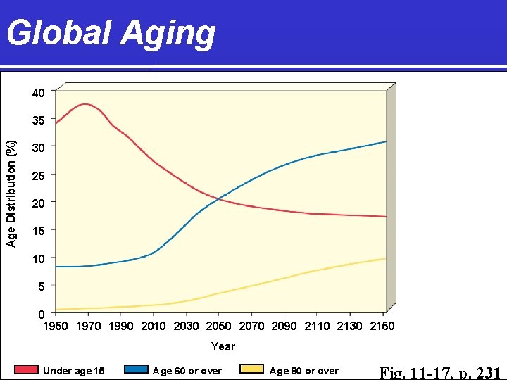
Global Aging 40 Age Distribution (%) 35 30 25 20 15 10 5 0 1950 1970 1990 2010 2030 2050 2070 2090 2110 2130 2150 Year Under age 15 Age 60 or over Age 80 or over Fig. 11 -17, p. 231
Solutions: Influencing Population Size Ø Migration Ø Reducing births Ø Economic development Ø Demographic transition Ø Family planning Ø Empowering women Ø Economic rewards and penalties
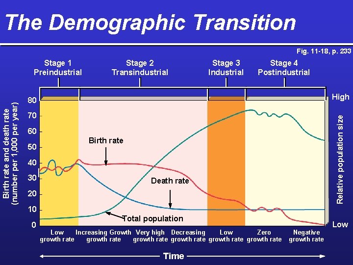
The Demographic Transition Fig. 11 -18, p. 233 Stage 2 Transindustrial Stage 3 Industrial Stage 4 Postindustrial High 80 70 Relative population size Birth rate and death rate (number per 1, 000 per year) Stage 1 Preindustrial 60 50 Birth rate 40 30 Death rate 20 10 0 Total population Low Increasing Growth Very high Decreasing Low Zero growth rate growth rate Time Low Negative growth rate
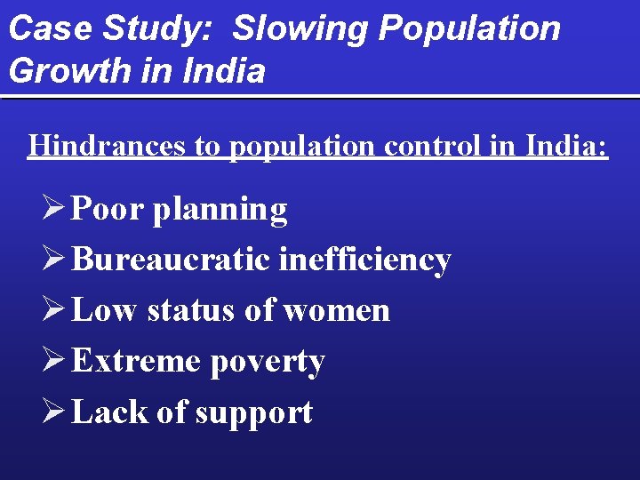
Case Study: Slowing Population Growth in India Hindrances to population control in India: Ø Poor planning Ø Bureaucratic inefficiency Ø Low status of women Ø Extreme poverty Ø Lack of support
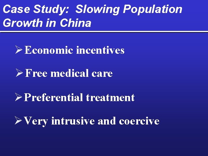
Case Study: Slowing Population Growth in China Ø Economic incentives Ø Free medical care Ø Preferential treatment Ø Very intrusive and coercive
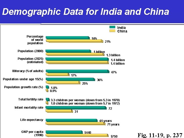
Demographic Data for India and China India China Percentage of world population 16% Population (2000) 21% 1 billion Population (2025) (estimated) 1. 3 billion 1. 4 billion Illiteracy (%of adults) 47% 17% Population under age 15(%) 36% 25% Population growth rate (%) Total fertility rate 1. 8% 0. 9% 3. 3 children per woman (down from 5. 3 in 1970) 1. 8 children per woman (down from 5. 7 in 1972) Infant mortality rate 72 31 Life expectancy GNP per capita (1998) 61 years 71 years $440 $750 Fig. 11 -19, p. 237
Cutting Global Population Growth Ø Family planning Ø Improve health care Ø Develop national population policies Ø Elevate the status of women Ø Increase education Ø Involve men in parenting Ø Reduce poverty Ø Sustainability
Urbanization and Urban Growth Ø Urban areas Ø Rural areas Ø Degree of urbanization Ø Urban growth: natural increase and immigration Ø Patterns of urbanization
Patterns of Urban Growth Ø Increasing proportion of population Ø Great increase in large cities (>1, 000) Ø Increasing rapidly in developing counties Ø Urban growth slower in developed countries Ø Poverty in urban areas increasing Ø Poverty, crime and pollution in Mexico City
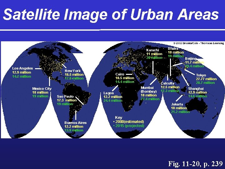
Satellite Image of Urban Areas Karachi 11 million 20 million Los Angeles 12. 9 million 14. 2 million Mexico City 18 million 19 million New York 16. 5 million 17. 6 million Sao Paulo 17. 3 million 19 million Buenos Aires 12. 2 million 13. 9 million Cairo 10. 5 million 14. 4 million Lagos 12. 2 million 24. 4 million Dhaka 10 million 19 million Calcutta 12. 5 million Mumbai (Bombay) 17. 3 million 18 million 27. 4 million Beijing 11. 7 million 19. 4 million Tokyo 27. 77 million 28. 7 million Shanghai 12. 9 million 14. 6 million Jakarta 10 million 21. 2 million Key • 2000(estimated) • 2015 (projected) Fig. 11 -20, p. 239
Urbanization in the US Ø Migration to large central cities Ø Migration from cities to suburbs Ø Migration from north and east to south and west Ø Migration from urban to rural areas Ø Spatial patterns of development

Two US Megalopolises Boston Springfield Hartford Providence Newark Allentown Harrisburg Baltimore New York Philadelphia Fig. 11 -21, p. 240 Washington Detroit Bowash (Boston to Washington) Chicago Toledo Cleveland Pittsburgh Akron Chipitts (Chicago to Pittsburgh)

Satellite Image of US Fig. 11 -22 a, p. 241
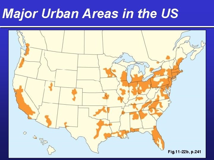
Major Urban Areas in the US Fig. 11 -22 b, p. 241
Advantages of Urbanization (especially in Developed Countries) Ø Economic advantages Ø Better access to health care Ø Environmental advantages Ø Biodiversity
Urban Problems Ø Resource use and waste (inputs and outputs) Ø Reduction in vegetation Ø Water supply problems and flooding Ø Air, noise, and water pollution Ø Disease, crime and accidents Ø Microclimates: Urban heat island Ø Impacts on surrounding rural areas
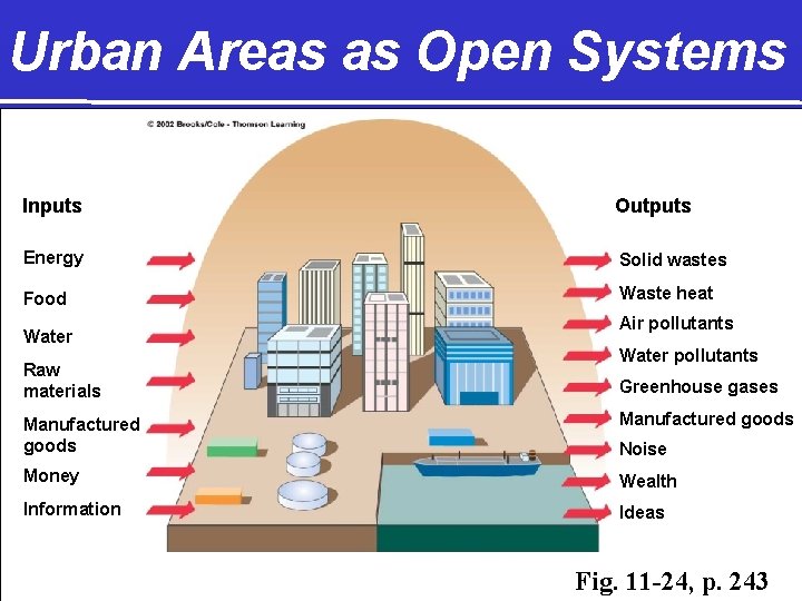
Urban Areas as Open Systems Inputs Outputs Energy Solid wastes Food Waste heat Water Raw materials Air pollutants Water pollutants Greenhouse gases Manufactured goods Money Wealth Information Ideas Noise Fig. 11 -24, p. 243
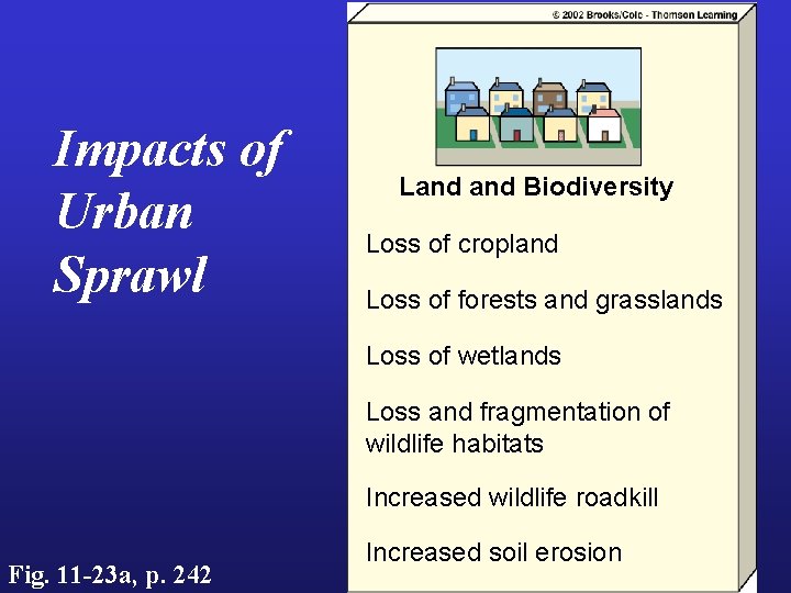
Impacts of Urban Sprawl Land Biodiversity Loss of cropland Loss of forests and grasslands Loss of wetlands Loss and fragmentation of wildlife habitats Increased wildlife roadkill Fig. 11 -23 a, p. 242 Increased soil erosion
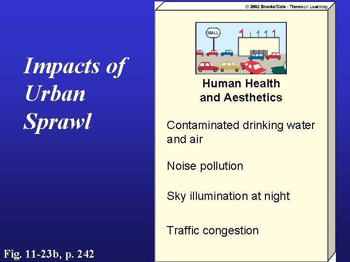
Impacts of Urban Sprawl Human Health and Aesthetics Contaminated drinking water and air Noise pollution Sky illumination at night Traffic congestion Fig. 11 -23 b, p. 242
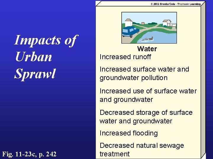
Impacts of Urban Sprawl Water Increased runoff Increased surface water and groundwater pollution Increased use of surface water and groundwater Decreased storage of surface water and groundwater Increased flooding Fig. 11 -23 c, p. 242 Decreased natural sewage treatment
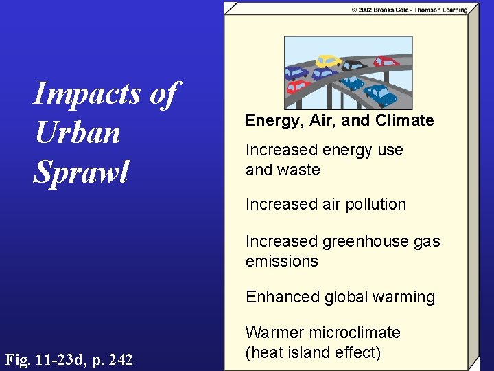
Impacts of Urban Sprawl Energy, Air, and Climate Increased energy use and waste Increased air pollution Increased greenhouse gas emissions Enhanced global warming Fig. 11 -23 d, p. 242 Warmer microclimate (heat island effect)
Impacts of Urban Sprawl Economic Effects Higher taxes Decline of downtown business districts Increased unemployment in central city Loss of tax base in central city Fig. 11 -23 e, p. 242
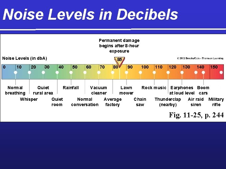
Noise Levels in Decibels Permanent damage begins after 8 -hour exposure Noise Levels (in db. A) 0 10 20 30 85 40 50 60 70 80 90 100 110 120 130 140 150 Normal Quiet Rainfall Vacuum Lawn Rock music Earphones Boom breathing rural area cleaner mower at loud level cars Whisper Quiet Normal Average Chain Thunderclap Air raid Military room conversation factory saw (nearby) siren rifle Fig. 11 -25, p. 244
Transportation and Urban Development Ø Individual transit Ø Mass transit Ø Land availability Ø Consequences of compact and dispersed cities Ø Role of motor vehicles in the US Ø Trade-offs of automobiles Ø Reduction of automobile use Ø Alternatives to automobiles
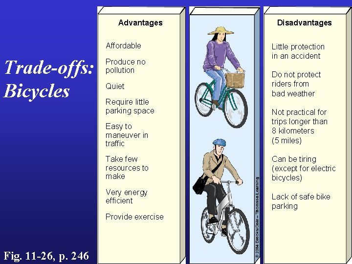
Advantages Affordable Trade-offs: Bicycles Produce no pollution Quiet Require little parking space Little protection in an accident Do not protect riders from bad weather Easy to maneuver in traffic Not practical for trips longer than 8 kilometers (5 miles) Take few resources to make Can be tiring (except for electric bicycles) Very energy efficient Provide exercise Fig. 11 -26, p. 246 Disadvantages Lack of safe bike parking
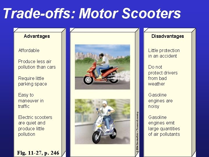
Trade-offs: Motor Scooters Advantages Affordable Produce less air pollution than cars Disadvantages Little protection in an accident Require little parking space Do not protect drivers from bad weather Easy to maneuver in traffic Gasoline engines are noisy Electric scooters are quiet and produce little pollution Gasoline engines emit large quantities of air pollutants Fig. 11 -27, p. 246
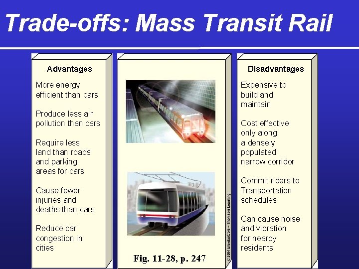
Trade-offs: Mass Transit Rail Advantages Disadvantages More energy efficient than cars Expensive to build and maintain Produce less air pollution than cars Cost effective only along a densely populated narrow corridor Require less land than roads and parking areas for cars Commit riders to Transportation schedules Cause fewer injuries and deaths than cars Can cause noise and vibration for nearby residents Reduce car congestion in cities Fig. 11 -28, p. 247
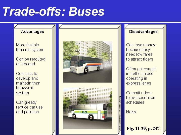
Trade-offs: Buses Advantages More flexible than rail system Can be rerouted as needed Cost less to develop and maintain than heavy-rail system Can greatly reduce car use and pollution Disadvantages Can lose money because they need low fares to attract riders Often get caught in traffic unless operating in express lanes Commit riders to transportation schedules Noisy Fig. 11 -29, p. 247
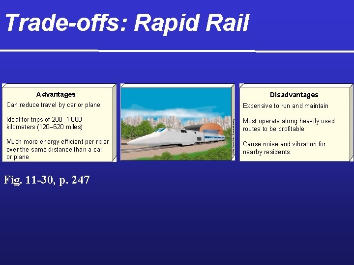
Trade-offs: Rapid Rail Advantages Disadvantages Can reduce travel by car or plane Expensive to run and maintain Ideal for trips of 200– 1, 000 kilometers (120– 620 miles) Must operate along heavily used routes to be profitable Much more energy efficient per rider over the same distance than a car or plane Cause noise and vibration for nearby residents Fig. 11 -30, p. 247
Making Urban Areas More Livable and Sustainable Ø Land-use planning Ø Property tax issues Ø Ecological land-use planning Ø Smart growth Ø Ecocities (Curitiba, Brazil)
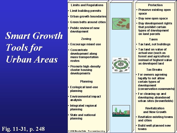
Limits and Regulations • Limit building permits • Urban growth boundaries • Green belts around cities Smart Growth Tools for Urban Areas • Public review of new development Zoning • Preserve existing open space • Buy new open space • Buy development rights that prohibit certain types of development on land parcels Taxes • Encourage mixed use • Tax land, not buildings • Concentrate development along mass transportation routes • Tax land on value of actual use (such as forest and agriculture) instead of highest value as developed land • Promote high-density cluster housing developments Planning • Ecological land-use planning • Environmental impact analysis • Integrated regional planning • State and national planning Fig. 11 -31, p. 248 Protection Tax Breaks • For owners agreeing legally to not allow certain types of development (conservation easements) • For cleaning up and developing abandoned urban sites (brownfields) Revitalization and New Growth • Revitalize existing towns and cities • Build well-planned new towns
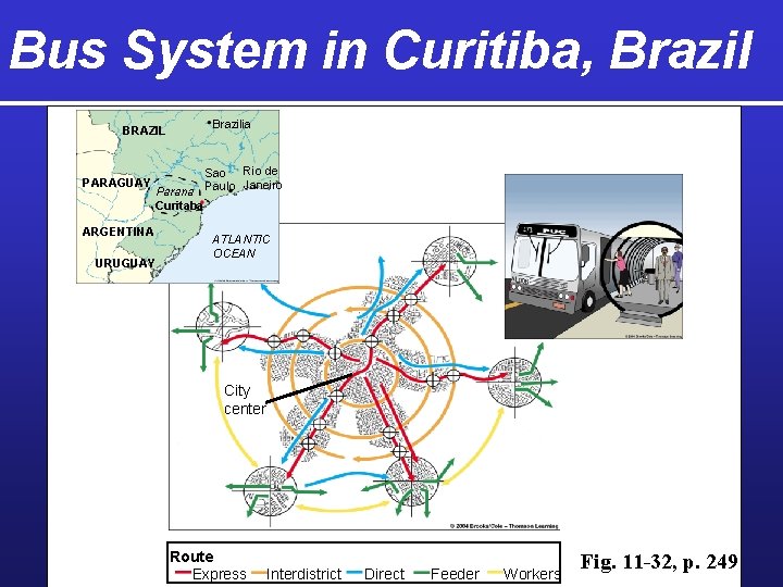
Bus System in Curitiba, Brazil BRAZIL PARAGUAY Brazilia Sao Rio de Janeiro Parana Paulo Curitaba ARGENTINA URUGUAY ATLANTIC OCEAN City center Route Express Interdistrict Direct Feeder Workers Fig. 11 -32, p. 249
- Slides: 62