The Hector Model current status and future plans

The Hector Model: current status and future plans Corinne A. Hartin Ben Bond-Lamberty Leon Clarke Joint Global Change Research Institute December 13, 2013 1

Model: motivation for Hector Fast executing simple global climate model an adaptive-timestep solver object-oriented coupler - easily swap in and out model components Interactive carbon chemistry in surface ocean Reproduce first-order responses of carbon and energy budgets from observations and GCMs MAGICC in particular has been heavily used across many scientific and policy communities & many strengths old difficult code to work with not open source, legal encumbrances unclear 2

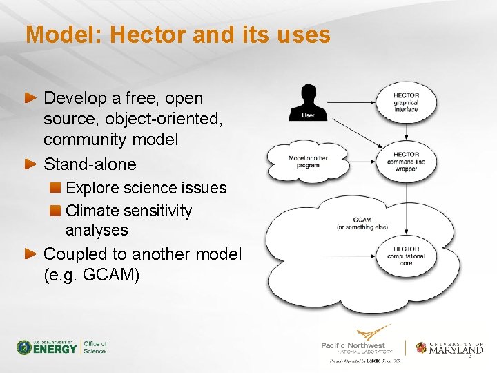
Model: Hector and its uses Develop a free, open source, object-oriented, community model Stand-alone Explore science issues Climate sensitivity analyses Coupled to another model (e. g. GCAM) 3

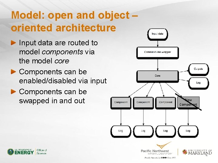
Model: open and object – oriented architecture Input data are routed to model components via the model core Components can be enabled/disabled via input Components can be swapped in and out New Component 4

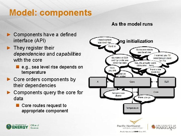
Model: components Components have a defined interface (API) They register their dependencies and capabilities with the core e. g. , sea level rise depends on temperature Core orders components by their dependencies Components query the core for data Core routes request to appropriate component 5

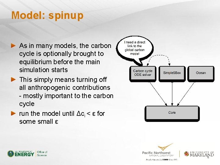
Model: spinup As in many models, the carbon cycle is optionally brought to equilibrium before the main simulation starts This simply means turning off all anthropogenic contributions - mostly important to the carbon cycle run the model until Δci < ε for some small ε 6

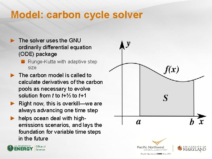
Model: carbon cycle solver The solver uses the GNU ordinarily differential equation (ODE) package Runge-Kutta with adaptive step size The carbon model is called to calculate derivatives of the carbon pools as necessary to evolve solution from t to t+½ to t+1 Right now, this is overkill—we are always advancing one time step helps ocean deal with highemissions scenarios, and lays the foundation for variable time steps in the future 7

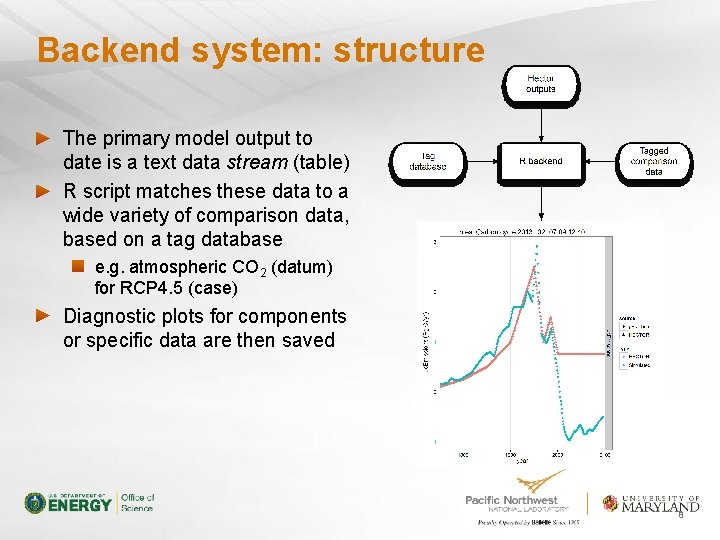
Backend system: structure The primary model output to date is a text data stream (table) R script matches these data to a wide variety of comparison data, based on a tag database e. g. atmospheric CO 2 (datum) for RCP 4. 5 (case) Diagnostic plots for components or specific data are then saved 8

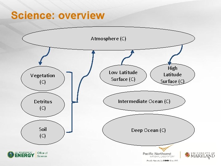
Science: overview Atmosphere (C) Vegetation (C) Detritus (C) Soil (C) Low Latitude Surface (C) High Latitude Surface (C) Intermediate Ocean (C) Deep Ocean (C) 9

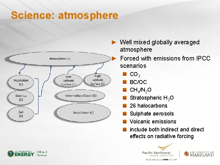
Science: atmosphere Well mixed globally averaged atmosphere Forced with emissions from IPCC scenarios CO 2 BC/OC CH 4/N 2 O Stratospheric H 2 O 26 halocarbons Sulphate aerosols Volcanic emissions include both indirect and direct effects on radiative forcing

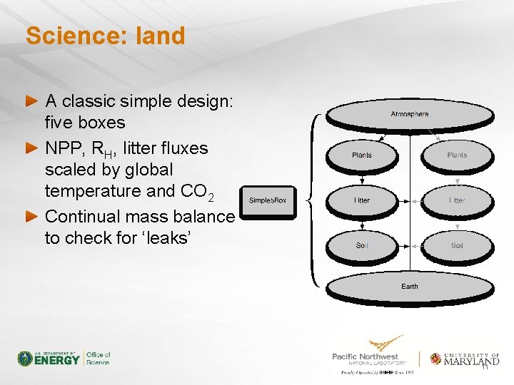
Science: land A classic simple design: five boxes NPP, RH, litter fluxes scaled by global temperature and CO 2 Continual mass balance to check for ‘leaks’ 11

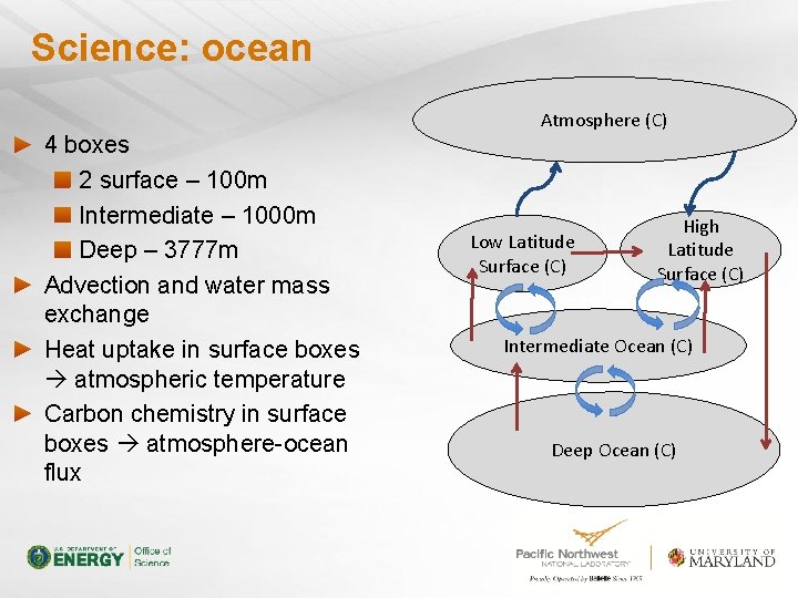
Science: ocean 4 boxes 2 surface – 100 m Intermediate – 1000 m Deep – 3777 m Advection and water mass exchange Heat uptake in surface boxes atmospheric temperature Carbon chemistry in surface boxes atmosphere-ocean flux Atmosphere (C) Low Latitude Surface (C) High Latitude Surface (C) Intermediate Ocean (C) Deep Ocean (C)

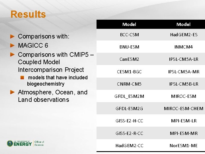
Results Model BCC-CSM Had. GEM 2 -ES BNU-ESM INMCM 4 Comparisons with: MAGICC 6 Comparisons with CMIP 5 – Coupled Model Intercomparison Project Can. ESM 2 IPSL-CM 5 A-LR CESM 1 -BGC IPSL-CM 5 A-MR models that have included biogeochemistry CNRM-CM 5 IPSL-CM 5 B-LR GFDL_ESM 2 M MIROC-ESM GFDL-ESM 2 G MIROC-ESM-CHEM GISS-E 2 -H-CC MPI-ESM-LR GISS-E 2 -R-CC MPI-ESM-MR Had. GEM 2 -CC Nor. ESM 1 -ME Atmosphere, Ocean, and Land observations

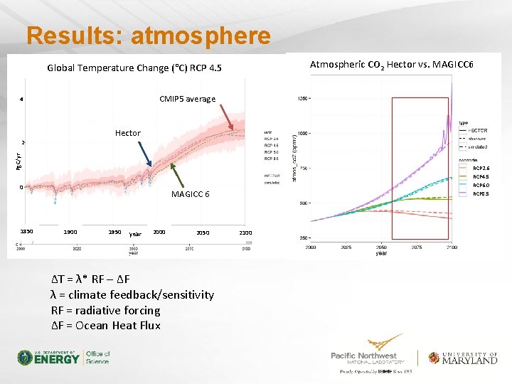
Results: atmosphere Global Temperature Change (°C) 4. 5 Global Temperature Change (°C) RCP Atmospheric CO CO 22 Hector vs. MAGICC 6 MAGICC Atmospheric CMIP 5 average 4 Hector Pg. C/yr 2 RCP 2. 6 RCP 4. 5 RCP 6. 0 0 1850 MAGICC 6 1900 1950 year 2000 2050 ΔT = λ* RF – ΔF λ = climate feedback/sensitivity RF = radiative forcing ΔF = Ocean Heat Flux RCP 8. 5 2100

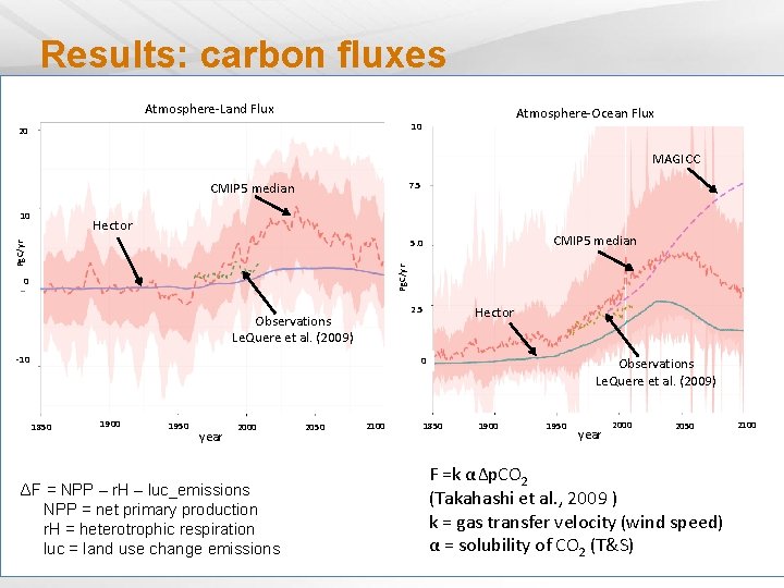
Results: carbon fluxes Atmosphere-Land Flux Atmosphere-Ocean Flux 10 20 MAGICC 7. 5 CMIP 5 median 10 Hector CMIP 5 median Pg. C/yr 5. 0 0 2. 5 Observations Le. Quere et al. (2009) -10 Hector 0 1850 1900 1950 year 2000 ΔF = NPP – r. H – luc_emissions NPP = net primary production r. H = heterotrophic respiration luc = land use change emissions 2050 2100 Observations Le. Quere et al. (2009) 1850 1900 1950 year 2000 2050 F =k αΔp. CO 2 (Takahashi et al. , 2009 ) k = gas transfer velocity (wind speed) α = solubility of CO 2 (T&S) 2100

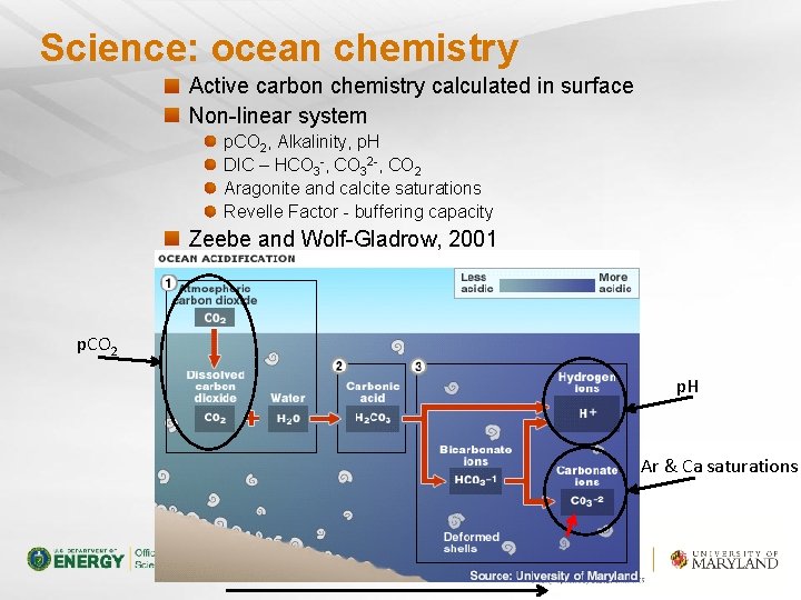
Science: ocean chemistry Active carbon chemistry calculated in surface Non-linear system p. CO 2, Alkalinity, p. H DIC – HCO 3 -, CO 32 -, CO 2 Aragonite and calcite saturations Revelle Factor - buffering capacity Zeebe and Wolf-Gladrow, 2001 p. CO 2 p. H Ar & Ca saturations

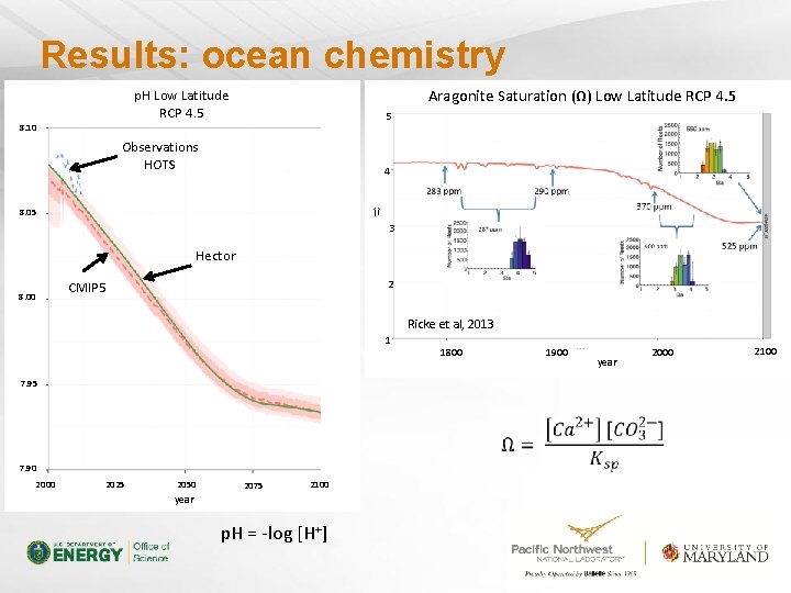
Results: ocean chemistry Aragonite Saturation (Ω) Low Latitude RCP 4. 5 p. H Low Latitude RCP 4. 5 5 8. 10 Observations HOTS 4 8. 05 3 Hector 8. 00 2 CMIP 5 Ricke et al, 2013 1 7. 95 7. 90 2000 2025 2050 2075 2100 year p. H = -log [H+] 1800 1900 year 2000 2100

Conclusions and Future Directions Simple climate box-model Open-source, community model Quick run times Simulates the general trends of MAGICC 6 and CMIP 5 Interactive carbon chemistry in the surface ocean - feedback on climate PSU Collaboration - Klaus Keller and Chris Forest Community model Engage students and post-docs Develop new components (to be switched in and out) Sea-ice Diffusive ocean - with more complex heat uptake Sea-level rise Detailed model-model comparisons Increase latitudinal resolution Varying albedo on both land ocean Organic carbon in ocean MCMC wrapper

Acknowledgments Pralit Patel, Robert Link, Steve Smith, Adria Schwarber – JGCRI Computer science and model development Klaus Keller and Chris Forest and others at Penn State model feedback and ideas DOE - IARP EPA