The HeckscherOhlin Model Features Flaws and Fixes II

The Heckscher-Ohlin Model: Features, Flaws, and Fixes II: What's Not to Like about the H -O Model Alan V. Deardorff University of Michigan

Themes of the 3 Lectures, Again • The HO Model is largely well behaved in 2 dimensions, even when you include trade costs Ø In higher dimensions, it is not so well behaved, especially when you include trade costs • Various modifications and extensions of the HO model offer some promise of making it behave better Nottingham II 2

Outline • Flaws of the HO Model – Minor Inconveniences of the 2× 2 Model – Major Inadequacies in Higher Dimensions • Indeterminacy of production and trade • Hypersensitivity to Trade Costs • Specialization – What Would a General Model Look Like? Nottingham II 3

Minor Inconveniences of the 2× 2 Model • The Prediction of Factor Price Equalization (FPE) – Ohlin’s belief in “only a tendency toward FPE” is • Wrong, in the exact version of the model that we have, but • Much easier to believe about the real world – But trade costs • Suffice to prevent complete FPE • Preserve tendency toward FPE in 2× 2 Model Nottingham II 4

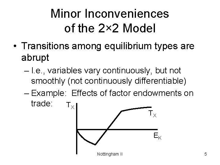
Minor Inconveniences of the 2× 2 Model • Transitions among equilibrium types are abrupt – I. e. , variables vary continuously, but not smoothly (not continuously differentiable) – Example: Effects of factor endowments on trade: TX TX EK Nottingham II 5

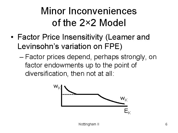
Minor Inconveniences of the 2× 2 Model • Factor Price Insensitivity (Leamer and Levinsohn’s variation on FPE) – Factor prices depend, perhaps strongly, on factor endowments up to the point of diversification, then not at all: w. K EK Nottingham II 6

Minor Inconveniences of the 2× 2 Model • Hard to apply to real world data – What are the two sectors? • Exports and imports? – What if they change? – Gross or net? • Capital- and labor-intensive goods? – How do you draw the line? – Both are traded both ways – What are the two factors? – If two countries, second country doesn’t match HO assumptions (e. g. , factor mobility) – Doesn’t allow for reality of intra-industry trade Nottingham II 7

Major Inadequacies in Higher Dimensions • These minor problems in two dimensions may suggest simply extending the HO Model to more goods, factors, and countries. – G goods, F factors, C countries Nottingham II 8

Major Inadequacies in Higher Dimensions • Immediate problem: – G > F → Production is indeterminate –G=F • Implausible • Not helpful (too many determinants of trade) –G<F • Specific factors model • Where did the specific factors come from? Nottingham II 9

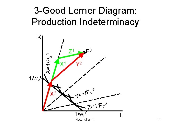
Major Inadequacies in Higher Dimensions • Production Indeterminacy – Enough to consider G=3, F=2 – If prices align so that all three goods can be produced, then infinitely many possible production patterns are possible – Implies indeterminacy of trade also – World market equilibrium does not resolve this (see Melvin 1968) Nottingham II 10

3 -Good Lerner Diagram: Production Indeterminacy X=1/PX 0 K Z 1 X 1 E 0 Y 2 1/w. K 0 X 2 0 1/P Y Y= 0 Z=1/P Z 1/w. L 0 Nottingham II L 11

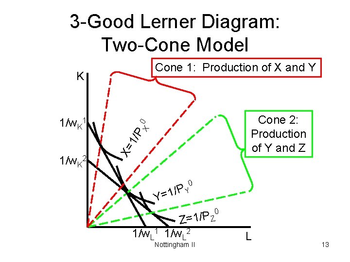
Major Inadequacies in Higher Dimensions • Production Indeterminacy – Alternative is prices that do not permit all three goods to be produced: Two-Cone HO Model Nottingham II 12

3 -Good Lerner Diagram: Two-Cone Model Cone 1: Production of X and Y 1/w. K 2 Cone 2: Production of Y and Z 1/P X= 1/w. K 1 X 0 K 0 1/P Y Y= 0 1/w. L 1 Z=1/P Z 1/w. L 2 Nottingham II L 13

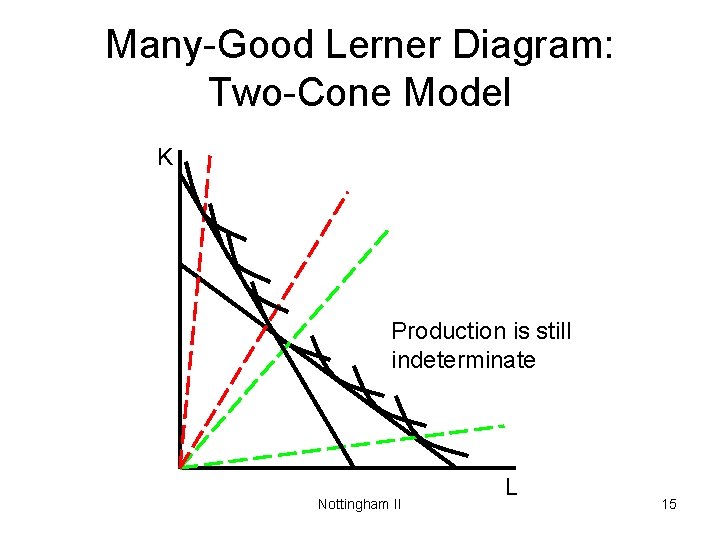
Major Inadequacies in Higher Dimensions • Production Indeterminacy – Two-cone model is attractive in many ways, • but with G>>F, there will be multiple goods in each cone, • and indeterminacy persists within cones. Nottingham II 14

Many-Good Lerner Diagram: Two-Cone Model K Production is still indeterminate Nottingham II L 15

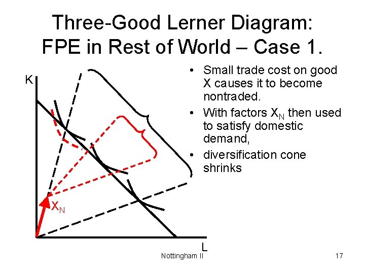
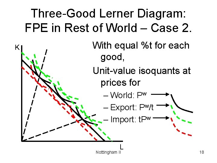
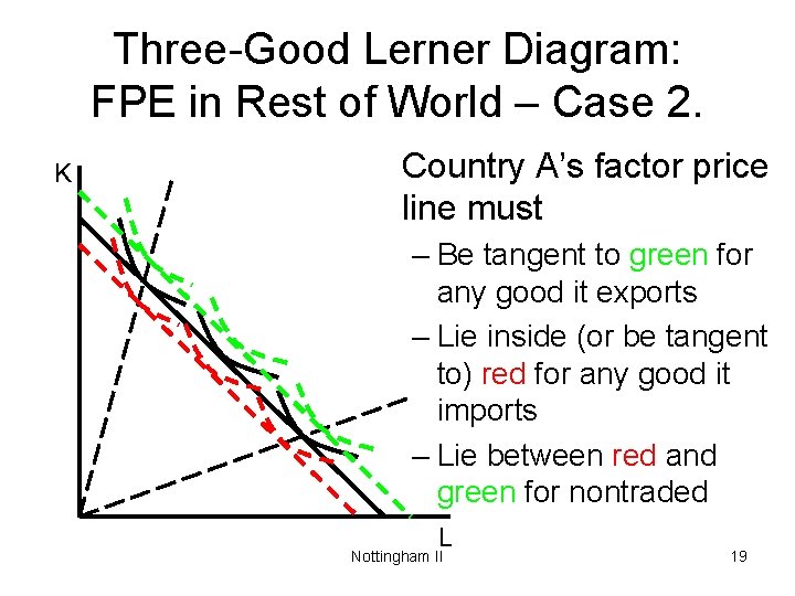
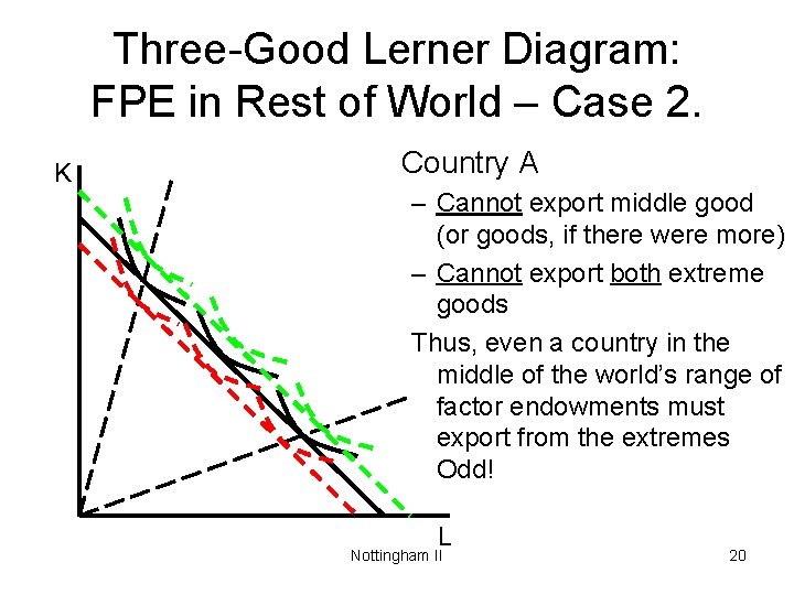
Can Trade Costs Help? • Yes, but they create other problems • Example 1: Suppose small country, A, trades with rest of world that has • More goods than factors • FPE • No trade costs – Then world prices align so that, without trade costs, production is indeterminate – Cases: 1. Country A has small trade cost, t, on just one good 2. Country A has equal % t on each good 3. Country A has unequal % t on each good Nottingham II 16

Three-Good Lerner Diagram: FPE in Rest of World – Case 1. • Small trade cost on good X causes it to become nontraded. • With factors XN then used to satisfy domestic demand, • diversification cone shrinks K XN L Nottingham II 17

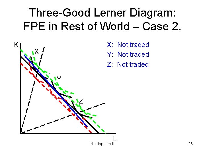
Three-Good Lerner Diagram: FPE in Rest of World – Case 2. K With equal %t for each good, Unit-value isoquants at prices for – World: Pw – Export: Pw/t – Import: t. Pw L Nottingham II 18

Three-Good Lerner Diagram: FPE in Rest of World – Case 2. K Country A’s factor price line must – Be tangent to green for any good it exports – Lie inside (or be tangent to) red for any good it imports – Lie between red and green for nontraded L Nottingham II 19

Three-Good Lerner Diagram: FPE in Rest of World – Case 2. K Country A – Cannot export middle good (or goods, if there were more) – Cannot export both extreme goods Thus, even a country in the middle of the world’s range of factor endowments must export from the extremes Odd! L Nottingham II 20

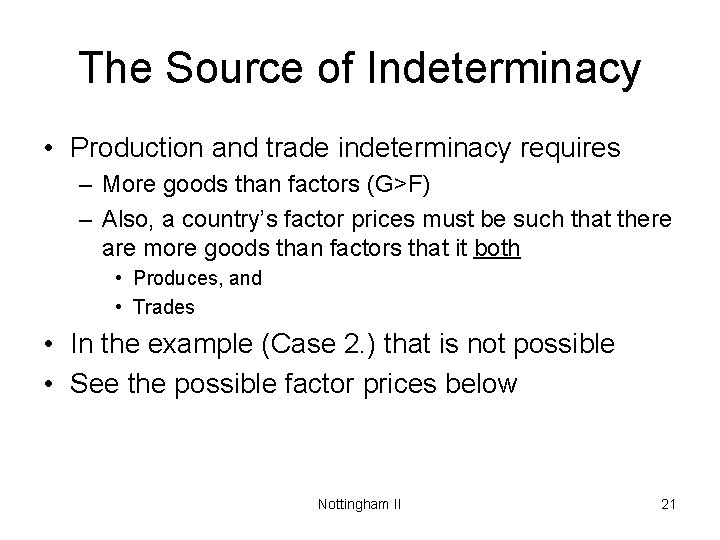
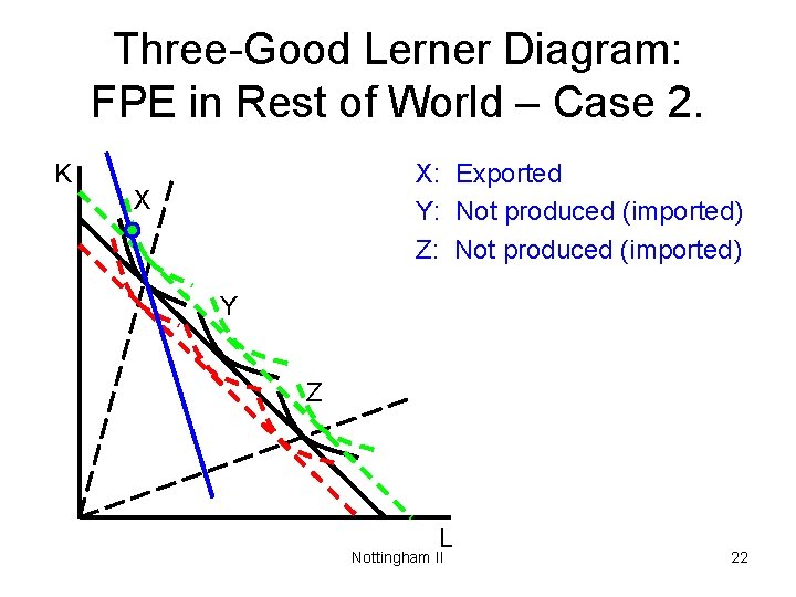
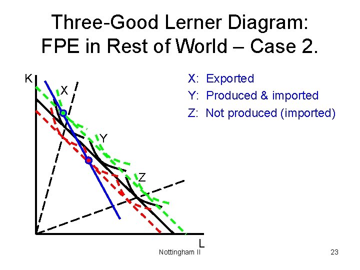
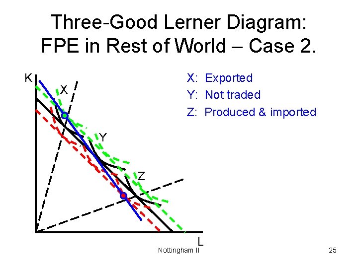
The Source of Indeterminacy • Production and trade indeterminacy requires – More goods than factors (G>F) – Also, a country’s factor prices must be such that there are more goods than factors that it both • Produces, and • Trades • In the example (Case 2. ) that is not possible • See the possible factor prices below Nottingham II 21

Three-Good Lerner Diagram: FPE in Rest of World – Case 2. K X: Exported Y: Not produced (imported) Z: Not produced (imported) X Y Z L Nottingham II 22

Three-Good Lerner Diagram: FPE in Rest of World – Case 2. K X: Exported Y: Produced & imported Z: Not produced (imported) X Y Z L Nottingham II 23

Three-Good Lerner Diagram: FPE in Rest of World – Case 2. K X: Exported Y: Not traded Z: Not produced (imported) X Y Z L Nottingham II 24

Three-Good Lerner Diagram: FPE in Rest of World – Case 2. K X: Exported Y: Not traded Z: Produced & imported X Y Z L Nottingham II 25

Three-Good Lerner Diagram: FPE in Rest of World – Case 2. K X: Not traded Y: Not traded Z: Not traded X Y Z L Nottingham II 26

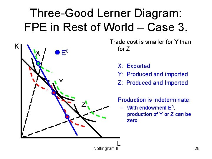
The Source of Indeterminacy • Can indeterminacy arise with G>F and trade costs? • Yes, but it requires trade costs and prices to align perfectly – This makes the indeterminacy itself “unlikely” – But it also implies that production and trade are “hypersensitive” to trade costs • See Example, Case 3. Nottingham II 27

Three-Good Lerner Diagram: FPE in Rest of World – Case 3. K X Trade cost is smaller for Y than for Z E 0 X: Exported Y: Produced and imported Z: Produced and Imported Y Z Production is indeterminate: – With endowment E 0, production of Y or Z can be zero L Nottingham II 28

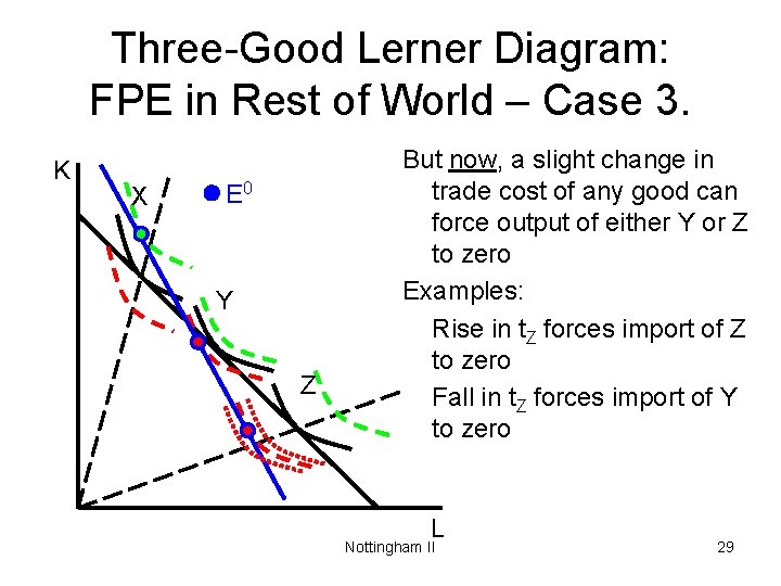
Three-Good Lerner Diagram: FPE in Rest of World – Case 3. K X E 0 Y Z But now, a slight change in trade cost of any good can force output of either Y or Z to zero Examples: Rise in t. Z forces import of Z to zero Fall in t. Z forces import of Y to zero L Nottingham II 29

Hypersensitivity to Trade Costs • This is just one example of how both production and trade in the HO model are very sensitive to trade costs: – Taking the model literally, an “epsilon” change in trade costs can cause positive trade and/or production to appear or disappear – Behavior is discontinuous in trade costs – I call this “hypersensitivity” Nottingham II 30

Hypersensitivity to Trade Costs • Causes of hypersensitivity that I’m aware of – Indeterminacy with G > F – Product homogeneity: Nobody cares with whom they trade, except for trade costs See Example 2 Nottingham II 31

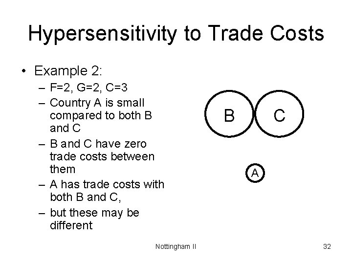
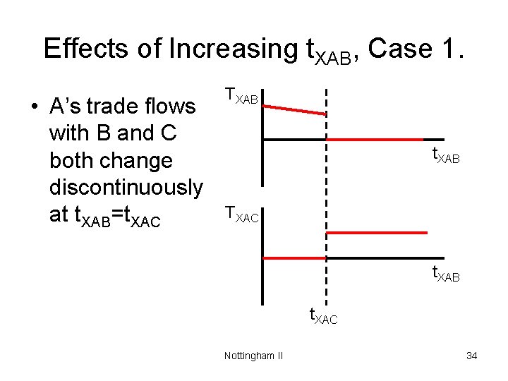
Hypersensitivity to Trade Costs • Example 2: – F=2, G=2, C=3 – Country A is small compared to both B and C – B and C have zero trade costs between them – A has trade costs with both B and C, – but these may be different Nottingham II B C A 32

Hypersensitivity to Trade Costs • Case 1: • B and C identical, thus same autarky prices • A is capital abundant compared to B and C, so A has comparative advantage in X – A will trade based on 2× 2 HO model, exporting X and importing Y – With whom A trades depends on trade costs • Let – TIJK be net export of good I from country J to country K, and – t. IJK be iceberg transport cost for that trade flow Nottingham II 33

Effects of Increasing t. XAB, Case 1. • A’s trade flows with B and C both change discontinuously at t. XAB=t. XAC TXAB t. XAB TXAC t. XAB t. XAC Nottingham II 34

Hypersensitivity to Trade Costs • Case 2: – If B and C have different factor endowments, but still no trade cost between them, then • A’s comparative advantage depends on its autarky price relative to B and C’s free trade price • Again, who it trades with depends discontinuously on its bilateral trade costs • (But having these trade costs differ is a bit weird, given the zero trade cost between them) Nottingham II 35

Hypersensitivity to Trade Costs • Case 3: – If B and C have different factor endowments, and trade costs between them, then • A’s comparative advantage can depend on its factor endowments relative to just B or C, depending on which it is closest to (“Local Comparative Advantage”) • Here the response of trade (that is, of what A trades as well as with whom) to trade costs does not seem to be hypersensitive Nottingham II 36

Specialization • With multiple countries, HO Model with trade costs predicts relatively few bilateral trade flows • This cannot be seen in the 2× 2× 2 model, where so few are possible • As number of countries grows, number of possible bilateral trade flows grows with square of C. Maximum number of equilibrium trade flows (except with zero probability) grows only with C. Nottingham II 37

Specialization • Argument – Suppose first that all factor prices and all trade costs are arbitrary (random) – Factor prices • Determine production costs in each country • And together with trade costs determine prices of exports to each other country – In equilibrium each country • Imports each good only from the one lowest cost other country (countries tie only with zero probability) • Or does not import a good at all, buying only from itself Nottingham II 38

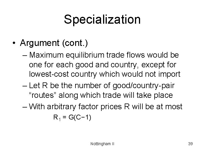
Specialization • Argument (cont. ) – Maximum equilibrium trade flows would be one for each good and country, except for lowest-cost country which would not import – Let R be the number of good/country-pair “routes” along which trade will take place – With arbitrary factor prices R will be at most R 1 = G(C− 1) Nottingham II 39

Specialization • Argument (cont. ) – But factor prices are not arbitrary: they adjust to achieve equilibrium – Suppose that they adjust, • Not to achieve equilibrium in factor markets, • But to achieve the largest number of possible equilibrium active trade routes – That would require equating export prices (production cost plus trade cost) of additional countries in destination countries – For each trade route that is not active with arbitrary factor prices, adjustment now seeks an equation of its export price with the price that is active Nottingham II 40

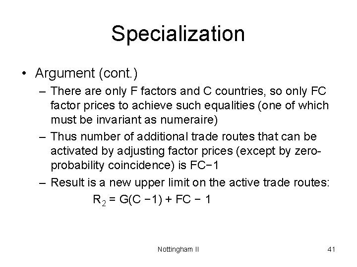
Specialization • Argument (cont. ) – There are only F factors and C countries, so only FC factor prices to achieve such equalities (one of which must be invariant as numeraire) – Thus number of additional trade routes that can be activated by adjusting factor prices (except by zeroprobability coincidence) is FC− 1 – Result is a new upper limit on the active trade routes: R 2 = G(C − 1) + FC − 1 Nottingham II 41

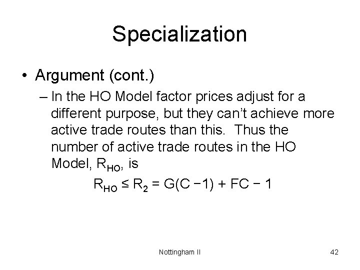
Specialization • Argument (cont. ) – In the HO Model factor prices adjust for a different purpose, but they can’t achieve more active trade routes than this. Thus the number of active trade routes in the HO Model, RHO, is RHO ≤ R 2 = G(C − 1) + FC − 1 Nottingham II 42

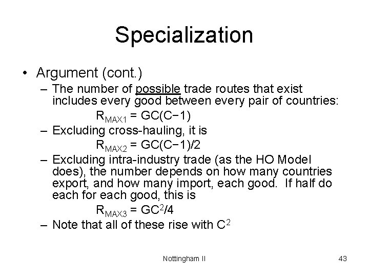
Specialization • Argument (cont. ) – The number of possible trade routes that exist includes every good between every pair of countries: RMAX 1 = GC(C− 1) – Excluding cross-hauling, it is RMAX 2 = GC(C− 1)/2 – Excluding intra-industry trade (as the HO Model does), the number depends on how many countries export, and how many import, each good. If half do each for each good, this is RMAX 3 = GC 2/4 – Note that all of these rise with C 2 Nottingham II 43

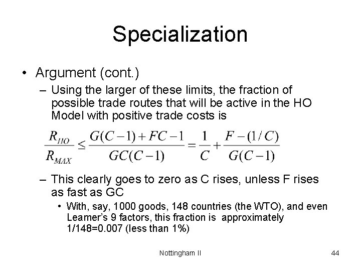
Specialization • Argument (cont. ) – Using the larger of these limits, the fraction of possible trade routes that will be active in the HO Model with positive trade costs is – This clearly goes to zero as C rises, unless F rises as fast as GC • With, say, 1000 goods, 148 countries (the WTO), and even Leamer’s 9 factors, this fraction is approximately 1/148=0. 007 (less than 1%) Nottingham II 44

Specialization • Argument (cont. ) – The argument is really about how many sources of supply there will be, and thus could be redone to include domestic supply. • Obviously we can’t predict that little will be supplied domestically, since high enough trade costs could lead to autarky • But the same kind of argument does suggest that the more that countries buy abroad, the less they will buy at home. Nottingham II 45

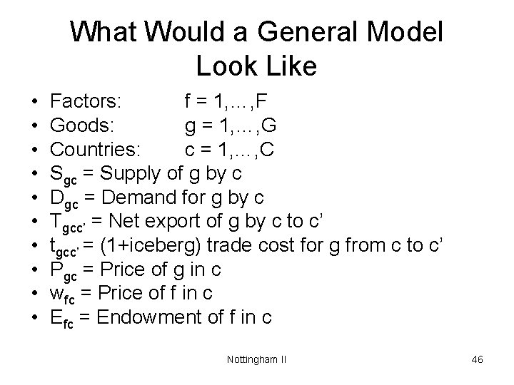
What Would a General Model Look Like • • • Factors: f = 1, …, F Goods: g = 1, …, G Countries: c = 1, …, C Sgc = Supply of g by c Dgc = Demand for g by c Tgcc’ = Net export of g by c to c’ tgcc’ = (1+iceberg) trade cost for g from c to c’ Pgc = Price of g in c wfc = Price of f in c Efc = Endowment of f in c Nottingham II 46

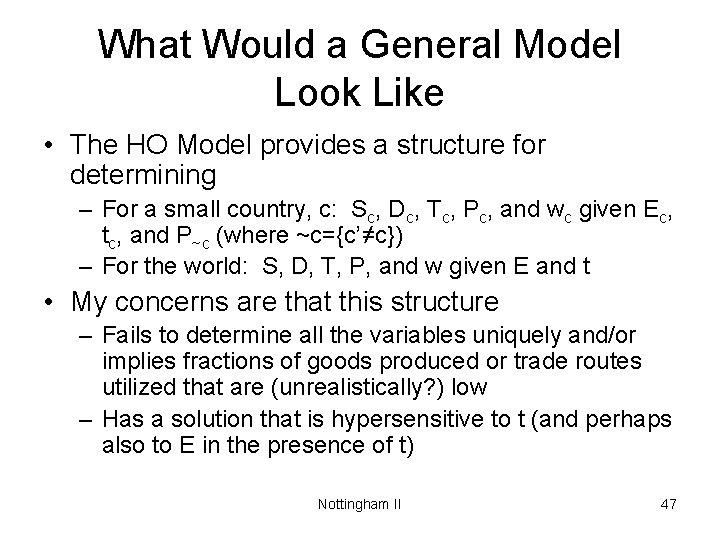
What Would a General Model Look Like • The HO Model provides a structure for determining – For a small country, c: Sc, Dc, Tc, Pc, and wc given Ec, tc, and P~c (where ~c={c’≠c}) – For the world: S, D, T, P, and w given E and t • My concerns are that this structure – Fails to determine all the variables uniquely and/or implies fractions of goods produced or trade routes utilized that are (unrealistically? ) low – Has a solution that is hypersensitive to t (and perhaps also to E in the presence of t) Nottingham II 47

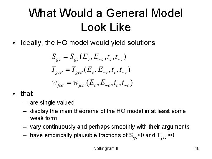
What Would a General Model Look Like • Ideally, the HO model would yield solutions • that – are single valued – display the main theorems of the HO model in at least some weak form – vary continuously and perhaps smoothly with their arguments – have empirically plausible fractions of Sgc>0 and Tgcc’>0 Nottingham II 48

What Would a General Model Look Like • The examples I’ve examined here suggest that this will not be possible under standard HO assumptions, especially if G>F and C>2. Nottingham II 49