The He LIx inversion code Genetic algorithms A

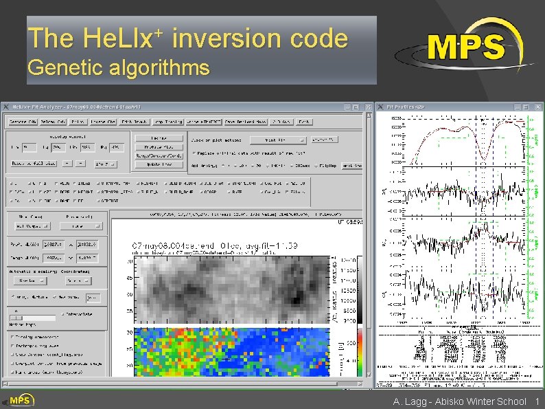
The He. LIx+ inversion code Genetic algorithms A. Lagg - Abisko Winter School 1

Inversion of the RTE Once solution of RTE is known: Ø comparison between Stokes spectra of synthetic and observed spectrum Ø trial-and-error changes of the initial parameters of the atmosphere („human inversions“) Ø until observed and synthetic (fitted) profile matches Inversions: Nothing else but an optimization of the trial-and-error part Problem: Inversions always find a solution within the given model atmosphere. Solution is seldomly unique (might even be completely wrong). Goal of this lecture: Principles of genetic algorithms Learn the usage of the He. LIx+ inversion code, develop a feeling on the reliability of inversion results. A. Lagg - Abisko Winter School 2

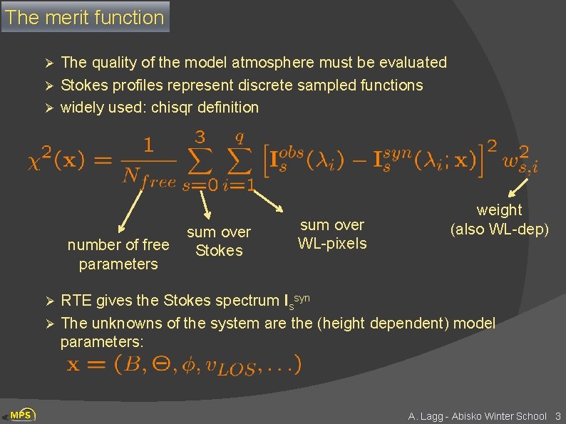
The merit function The quality of the model atmosphere must be evaluated Ø Stokes profiles represent discrete sampled functions Ø widely used: chisqr definition Ø number of free parameters sum over Stokes sum over WL-pixels weight (also WL-dep) RTE gives the Stokes spectrum Issyn Ø The unknowns of the system are the (height dependent) model parameters: Ø A. Lagg - Abisko Winter School 3

He. LIx+ overview of features includes Zeeman, Paschen-Back, Hanle effect (He 10830) atomic polarization for He 10830 (He D 3) magneto-optical effects fitting / removing telluric lines fitting unknown parameters of spectral lines various methods for continuum correction / fitting convolution with instrument filter profiles user-defined weighting scheme direct read access to SOT/SP, VTT-TIP 2, SST-CRISP, . . . flexible atomic data configuration extensive IDL based display routines MPI support (to invert maps) Download from http: //www. mps. mpg. de/homes/lagg GBSO download-section helix use invert and IR$soft A. Lagg - Abisko Winter School 4

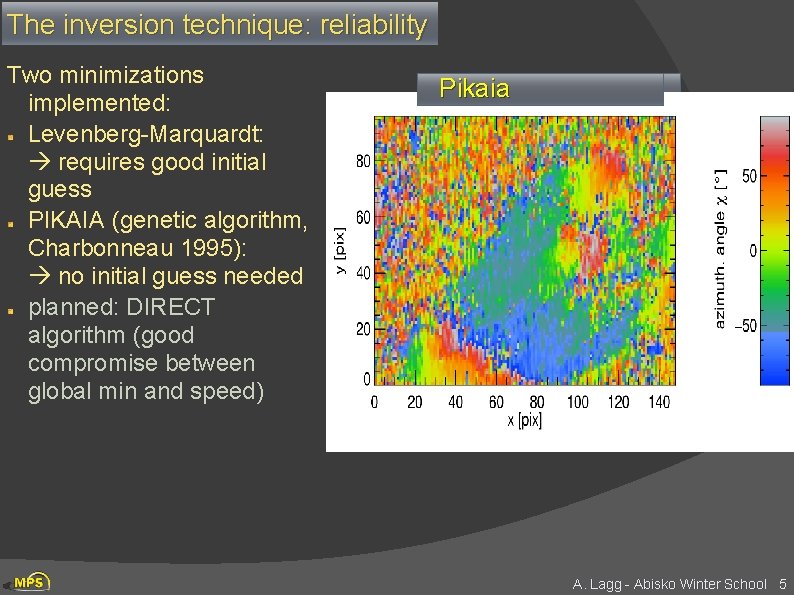
The inversion technique: reliability Two minimizations implemented: Levenberg-Marquardt: requires good initial guess PIKAIA (genetic algorithm, Charbonneau 1995): no initial guess needed planned: DIRECT algorithm (good compromise between global min and speed) steepest Pikaia gradient A. Lagg - Abisko Winter School 5

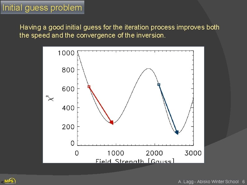
Initial guess problem Having a good initial guess for the iteration process improves both the speed and the convergence of the inversion. A. Lagg - Abisko Winter School 6

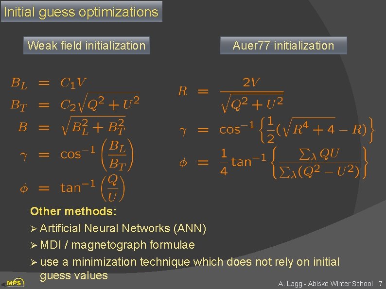
Initial guess optimizations Weak field initialization Auer 77 initialization Other methods: Ø Artificial Neural Networks (ANN) Ø MDI / magnetograph formulae Ø use a minimization technique which does not rely on initial guess values A. Lagg - Abisko Winter School 7

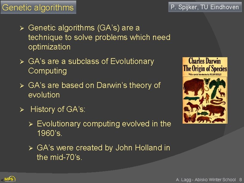
Genetic algorithms Ø Genetic algorithms (GA’s) are a technique to solve problems which need optimization Ø GA’s are a subclass of Evolutionary Computing Ø GA’s are based on Darwin’s theory of evolution Ø P. Spijker, TU Eindhoven History of GA’s: Ø Evolutionary computing evolved in the 1960’s. Ø GA’s were created by John Holland in the mid-70’s. A. Lagg - Abisko Winter School 8

Advantages / drawbacks Ø No derivatives of the goodness of fit function with respect to model parameters need be computed; it matters little whether the relationship between the model and its parameters is linear or nonlinear. Ø Nothing in the procedure outlined above depends critically on using a least-squares statistical estimator; any other robust estimator can be substituted, with little or no changes to the overall procedure. Ø In most real applications, the model will need to be evaluated (i. e. , given a parameter set, compute a synthetic dataset and its associated goodness of fit) a great many times; if this evaluation is computationally expensive, the forward modeling approach can become impractical. A. Lagg - Abisko Winter School 9

Evolution in biology Ø Each cell of a living thing contains chromosomes - strings of DNA Ø Each chromosome contains a set of genes - blocks of DNA Ø Each gene determines some aspect of the organism (like eye colour) Ø A collection of genes is sometimes called a genotype Ø A collection of aspects (like eye colour) is sometimes called a phenotype Ø Reproduction involves recombination of genes from parents and then small amounts of mutation (errors) in copying Ø The fitness of an organism is how much it can reproduce before it dies Ø Evolution based on “survival of the fittest” A. Lagg - Abisko Winter School 10

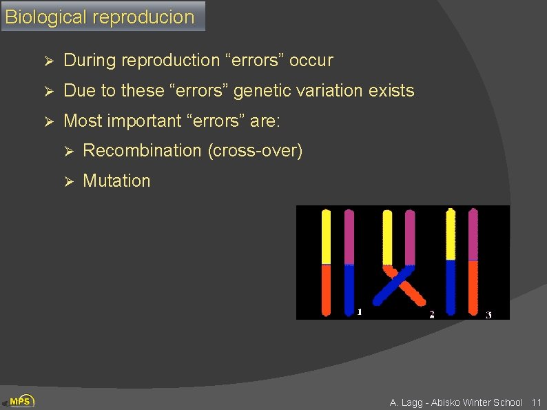
Biological reproducion Ø During reproduction “errors” occur Ø Due to these “errors” genetic variation exists Ø Most important “errors” are: Ø Recombination (cross-over) Ø Mutation A. Lagg - Abisko Winter School 11

Natural selection Ø The origin of species: “Preservation of favourable variations and rejection of unfavourable variations. ” Ø There are more individuals born than can survive, so there is a continuous struggle for life. Ø Individuals with an advantage have a greater chance for survive: survival of the fittest. Ø Important aspects in natural selection are: Ø adaptation to the environment Ø isolation of populations in different groups which cannot mutually mate Ø If small changes in the genotypes of individuals are expressed easily, especially in small populations, we speak of genetic drift Ø “success in life”: mathematically expressed as fitness A. Lagg - Abisko Winter School 12

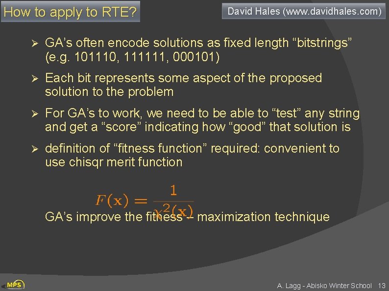
How to apply to RTE? David Hales (www. davidhales. com) Ø GA’s often encode solutions as fixed length “bitstrings” (e. g. 101110, 111111, 000101) Ø Each bit represents some aspect of the proposed solution to the problem Ø For GA’s to work, we need to be able to “test” any string and get a “score” indicating how “good” that solution is Ø definition of “fitness function” required: convenient to use chisqr merit function GA’s improve the fitness – maximization technique A. Lagg - Abisko Winter School 13

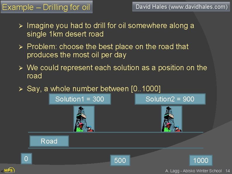
Example – Drilling for oil David Hales (www. davidhales. com) Ø Imagine you had to drill for oil somewhere along a single 1 km desert road Ø Problem: choose the best place on the road that produces the most oil per day Ø We could represent each solution as a position on the road Ø Say, a whole number between [0. . 1000] Solution 1 = 300 Solution 2 = 900 Road 0 500 1000 A. Lagg - Abisko Winter School 14

Encoding problem Ø The set of all possible solutions [0. . 1000] is called the search space or state space Ø In this case it’s just one number but it could be many numbers or symbols Ø Often GA’s code numbers in binary producing a bitstring representing a solution Ø In our example we choose 10 bits which is enough to represent 0. . 1000 512 256 128 64 32 16 8 4 2 1 900 1 1 1 0 0 300 0 1 0 1 1 0 0 1023 1 1 1 1 1 In GA’s these encoded strings are sometimes called “genotypes” or “chromosomes” and the individual bits are sometimes called “genes” A. Lagg - Abisko Winter School 15

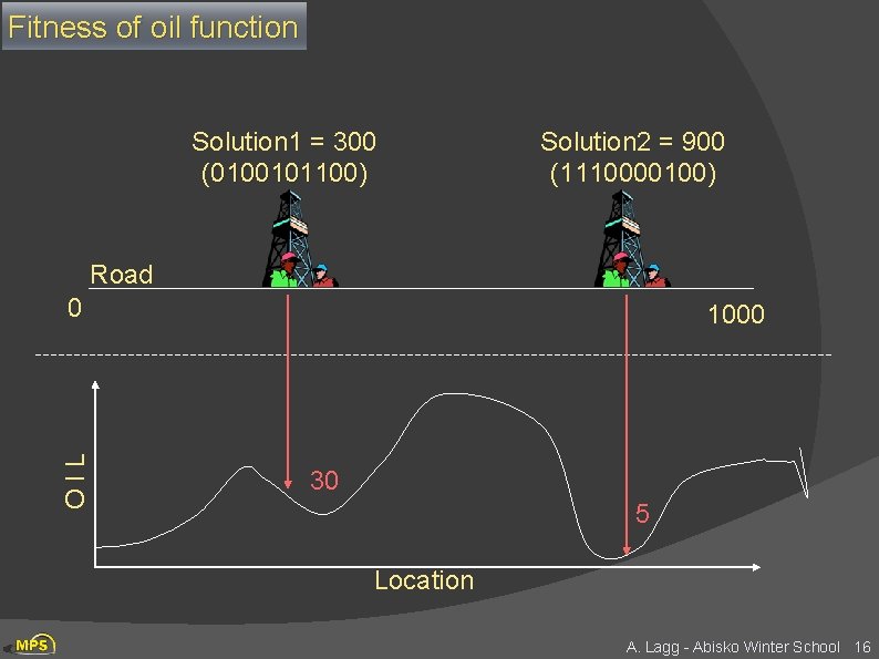
Fitness of oil function Solution 1 = 300 (0100101100) 0100101100 Solution 2 = 900 (1110000100) Road OIL 0 1000 30 5 Location A. Lagg - Abisko Winter School 16

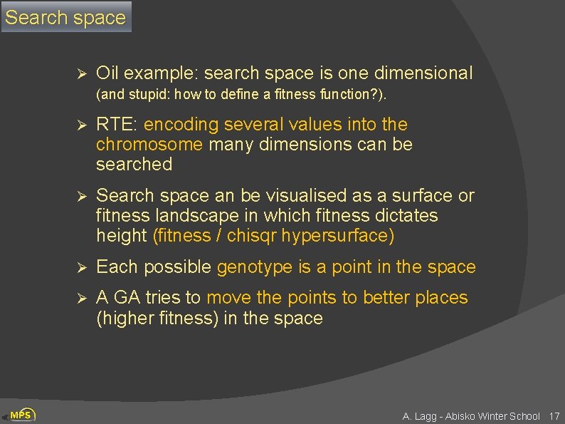
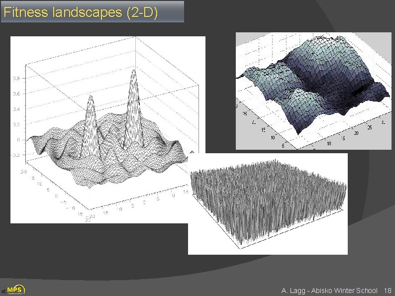
Search space Ø Oil example: search space is one dimensional (and stupid: how to define a fitness function? ). Ø RTE: encoding several values into the chromosome many dimensions can be searched Ø Search space an be visualised as a surface or fitness landscape in which fitness dictates height (fitness / chisqr hypersurface) Ø Each possible genotype is a point in the space Ø A GA tries to move the points to better places (higher fitness) in the space A. Lagg - Abisko Winter School 17

Fitness landscapes (2 -D) A. Lagg - Abisko Winter School 18

Search space Ø Obviously, the nature of the search space dictates how a GA will perform Ø A completely random space would be bad for a GA Ø Also GA’s can, in practice, get stuck in local maxima if search spaces contain lots of these Ø Generally, spaces in which small improvements get closer to the global optimum are good A. Lagg - Abisko Winter School 19

The algorithm Ø Generate a set of random solutions Ø Repeat Ø Ø Test each solution in the set (rank them) Ø Remove some bad solutions from set Ø Duplicate some good solutions Ø make small changes to some of them Until best solution is good enough How to duplicate good solutions? A. Lagg - Abisko Winter School 20

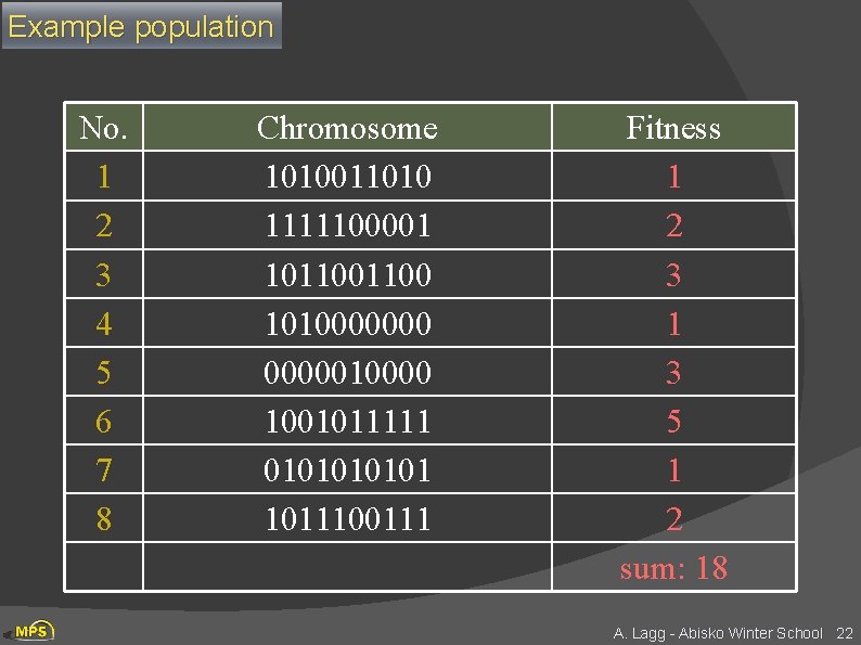
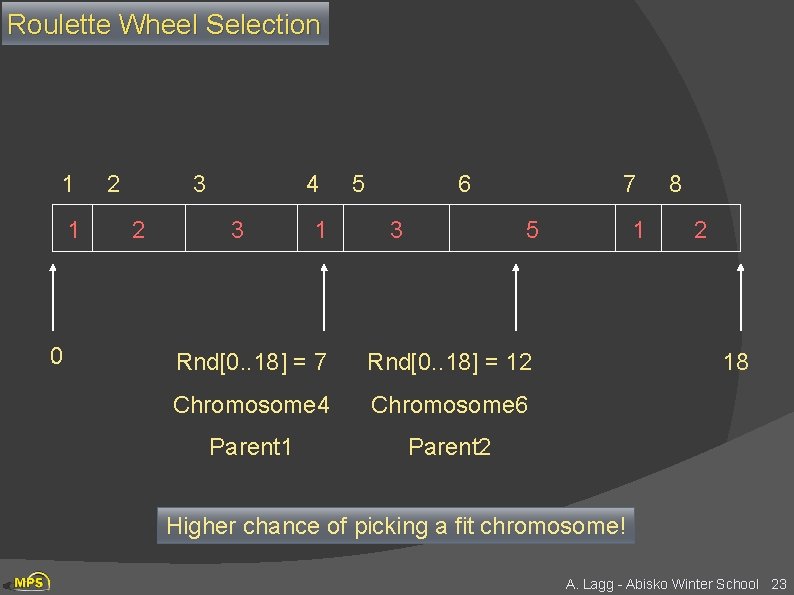
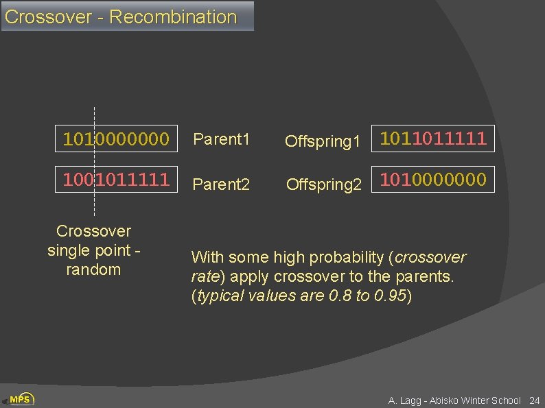
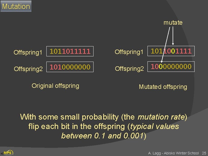
Adding Sex Ø Two high scoring “parent” bit strings (chromosomes) are selected and with some probability (crossover rate) combined sex Ø Producing two new offsprings (bit strings) result of sex Ø Each offspring may then be changed randomly (mutation) parents are seldom happy with the result Ø Selecting parents: many schemes possible, example: Roulette Wheel Ø Add up the fitness's of all chromosomes Ø Generate a random number R in that range Ø Select the first chromosome in the population that - when all previous fitness’s are added gives you at least the value R A. Lagg - Abisko Winter School 21

Example population No. 1 2 3 4 5 6 7 8 Chromosome 1010011010 1111100001 101100 101000000010000 1001011111 010101 1011100111 Fitness 1 2 3 1 3 5 1 2 sum: 18 A. Lagg - Abisko Winter School 22

Roulette Wheel Selection 1 1 0 2 3 2 4 3 1 5 6 3 7 5 Rnd[0. . 18] = 7 Rnd[0. . 18] = 12 Chromosome 4 Chromosome 6 Parent 1 Parent 2 1 8 2 18 Higher chance of picking a fit chromosome! A. Lagg - Abisko Winter School 23

Crossover - Recombination 1010000000 Parent 1 Offspring 1 1011011111 1001011111 Parent 2 Offspring 2 1010000000 Crossover single point random With some high probability (crossover rate) apply crossover to the parents. (typical values are 0. 8 to 0. 95) A. Lagg - Abisko Winter School 24

Mutation mutate Offspring 1 1011011111 Offspring 1 1011001111 Offspring 2 1010000000 Offspring 2 100000 Original offspring Mutated offspring With some small probability (the mutation rate) flip each bit in the offspring (typical values between 0. 1 and 0. 001) A. Lagg - Abisko Winter School 25

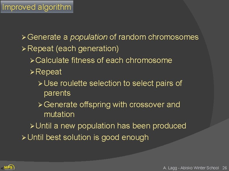
Improved algorithm Ø Generate a population of random chromosomes Ø Repeat (each generation) Ø Calculate fitness of each chromosome Ø Repeat Ø Use roulette selection to select pairs of parents Ø Generate offspring with crossover and mutation Ø Until a new population has been produced Ø Until best solution is good enough A. Lagg - Abisko Winter School 26

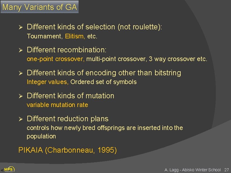
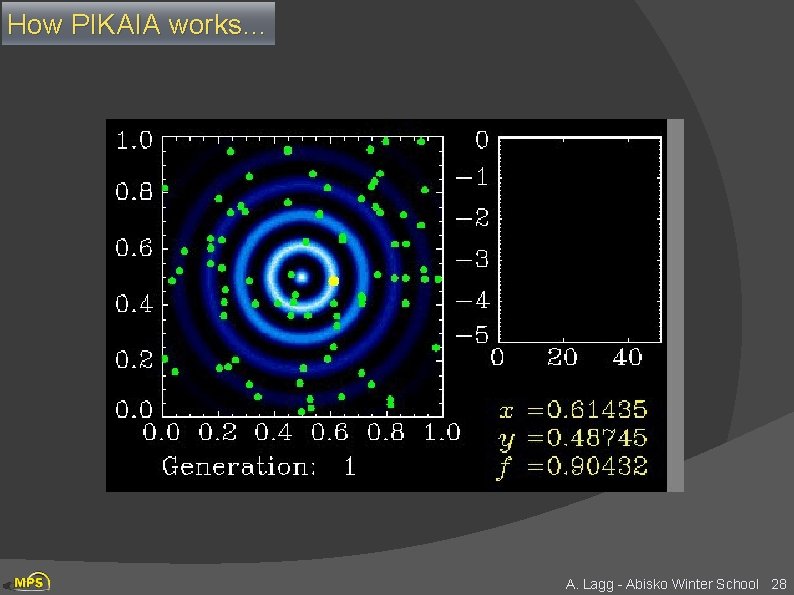
Many Variants of GA Ø Different kinds of selection (not roulette): Tournament, Elitism, etc. Ø Different recombination: one-point crossover, multi-point crossover, 3 way crossover etc. Ø Different kinds of encoding other than bitstring Integer values, Ordered set of symbols Ø Different kinds of mutation variable mutation rate Ø Different reduction plans controls how newly bred offsprings are inserted into the population PIKAIA (Charbonneau, 1995) A. Lagg - Abisko Winter School 27

How PIKAIA works… A. Lagg - Abisko Winter School 28

List of ME Codes (incomplete) Ø Ø Ø He. LIx+ A. Lagg, most flexible code (multi-comp, multi line), He 10830 Hanle slab model implemented. Genetic algorithm Pikaia. Fully parallel. VFISV J. M. Borrero, for SDO HMI. Fastest ME code available. F 90, fully parallel. Levenberg-Marquardt with some optimizations. MERLIN Written by Jose Garcia at HAO in C, C++ and some other routines in Fortran. (Lites et al. 2007 in Il Nouvo Cimento) MELANIE Hector Socas at HAO. In F 90, not parallel. Numerical derivatives. HAZEL Artoro Lopez Ariste et al. (2008). Optimized for He 10830, He D 3, Hanle-slab model. MILOS Orozco Suarez et al. (2007), IDL, some papers published with it A. Lagg - Abisko Winter School 29

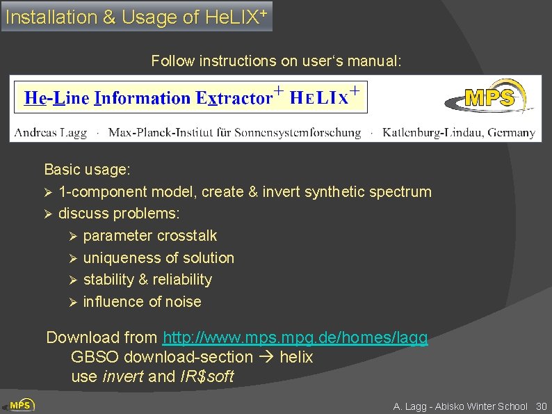
Installation & Usage of He. LIX+ Follow instructions on user‘s manual: Basic usage: Ø 1 -component model, create & invert synthetic spectrum Ø discuss problems: Ø parameter crosstalk Ø uniqueness of solution Ø stability & reliability Ø influence of noise Download from http: //www. mps. mpg. de/homes/lagg GBSO download-section helix use invert and IR$soft A. Lagg - Abisko Winter School 30

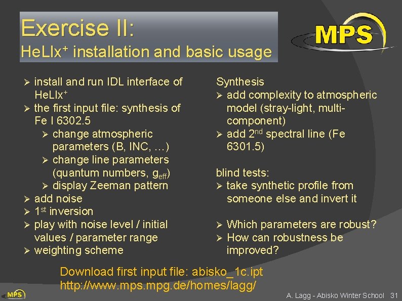
Exercise II: He. LIx+ installation and basic usage Ø Ø Ø install and run IDL interface of He. LIx+ the first input file: synthesis of Fe I 6302. 5 Ø change atmospheric parameters (B, INC, …) Ø change line parameters (quantum numbers, geff) Ø display Zeeman pattern add noise 1 st inversion play with noise level / initial values / parameter range weighting scheme Synthesis Ø add complexity to atmospheric model (stray-light, multicomponent) Ø add 2 nd spectral line (Fe 6301. 5) blind tests: Ø take synthetic profile from someone else and invert it Ø Ø Which parameters are robust? How can robustness be improved? Download first input file: abisko_1 c. ipt http: //www. mps. mpg. de/homes/lagg/ A. Lagg - Abisko Winter School 31