The Global Positioning System GPS and Satellite Time
 and Satellite Time Transfer Michael Lombardi NIST Time and")
The Global Positioning System (GPS) and Satellite Time Transfer Michael Lombardi NIST Time and Frequency Division SIM Time and Frequency Metrology Working Group Workshop and Planning Meeting Bogota, Colombia October 23 -26, 2017

Outline • Overview of GPS • Overview of how time is obtained from GPS • One-Way time transfer – - Uncertainty analysis of the one-way method • Common-view time transfer – - Uncertainty analysis of the common-view method • The SIM Time Network • Contributing to UTC by participating in the BIPM key comparisons • Other GNSS systems

Overview of GPS
 is best known for positioning")
What is GPS? § The Global Positioning System (GPS) is best known for positioning and navigation, but it is also the primary system used to distribute accurate time and frequency worldwide. It is operated by the United States Air Force. § The satellites are in semi-synchronous orbit at an altitude of about 20, 180 km § The orbital period is 11 hours, 58 minutes § At least four satellites, but typically seven or more, can always be received at a given location, so the entire Earth has continuous GPS coverage § The satellites each carry either cesium or rubidium atomic clocks (or both)
 numbers used to identify")
GPS Satellites • There are 32 pseudo random noise (PRN) numbers used to identify the GPS satellites, but the maximum number of operational satellites is 31. • At this writing (October 2017): ü There are 31 operational satellites, the maximum number. The SIM system (top right corner of screen) indicates which satellites have been received during the current UTC day. ü Only two satellites (PRN 8 and PRN 24) are referenced to cesium clocks, the others are referenced to rubidium clocks. ü The oldest satellite is PRN 13, launched in July 1997. ü The newest satellite is PRN 32, launched in February 2016.

GPS Signal Structure GPS Structure All GPS satellites use two L-band carrier frequencies L 1 = 1575. 42 MHz L 2 = 1227. 60 MHz The most recently launched satellites also broadcast – L 5 = 1176. 45 MHz, now on 12 satellites – L 2 C now on 19 satellites – L 1 C is coming, but not on any satellites yet Legacy PRN Codes broadcast by all satellites – P(Y): Military Code ü 267 day repeat interval ü Encrypted – code sequence not published ü Available on L 1 and L 2 – C/A: Coarse Acquisition (Civilian) Code ü 1 millisecond repeat interval ü Available to all users, but only on L 1 The new frequencies have new codes, but they are not implemented yet in many timing receivers – for example L 5 has the I 5 and Q 5 codes. The codes contain a navigation message that – – Provides ephemeris data and clock corrections for the GPS satellites Is transmitted at a low data rate (50 bits per second)

GPS Modulation ü The unmodulated GPS carrier is a sine wave. Two binary codes are modulated on to the sine wave: the C/A (coarse/acquisition) code and the P (precise) code. ü Binary biphase modulation (also known as binary phase shift keying [BPSK]) is the technique used to modulate the binary codes onto the carrier. There is a 180 degree carrier phase shift each time the code state changes. Unmodulated Carrier
![GPS Signal (L 1 band, C/A Code) P[d. BW] 2. 046 MHz C/A-CODE P-CODE](http://slidetodoc.com/presentation_image_h/e336de69c4fc1ff58478368b88d46db6/image-8.jpg "GPS Signal (L 1 band, C/A Code) P[d. BW] 2. 046 MHz C/A-CODE P-CODE")
GPS Signal (L 1 band, C/A Code) P[d. BW] 2. 046 MHz C/A-CODE P-CODE -160 -163 1575. 42 MHz P[d. BW] f [Hz] L 1 Signal 20. 46 MHz Frequency Spectrum n C/A stands for Coarse Acquisition. The C/A code, broadcast on the L 1 carrier at 1575. 42 MHz, is the reference for nearly all GPS consumer products, including the receivers used in the SIM Time Network. GPS spreads the data over a bandwidth much wider than needed to carry the small amount of information that is broadcast, allowing very low power signals to be used. This “spread spectrum” technique is the same principle now used by many household devices such as cordless phones, baby monitors, garage door openers, etc.

GPS Positioning • GPS positioning depends on: ü The precise measurement of time ü The constancy of the speed of light • GPS positioning is based on trilateration ü GPS satellite positions are known ü Receiver position is not known ü GPS-to-receiver range measurements are used to compute the receiver’s position

Positioning Example with One Transmitter Locus of points on which the receiver can be located Receiver (location unknown) Measured Range Transmitter (location known)

Positioning Example with Two Transmitters True Receiver Location r 1 T 1 r 2 T 2 False Receiver Location

Positioning Example with Three Transmitters True Receiver Location r 1 T 1 r 3 r 2 T 3

Solving for Receiver Position and Time • The position solution involves solving for four unknowns: ü Receiver position (x, y, z coordinates) ü Time • A positioning uncertainty of about 10 meters requires the time of the receiver clock to be known to within about 30 ns, because the speed of light is about 3 ns per meter. • The solution requires: ü Range measurements to each satellite to determine the signal propagation delay ü Reading the data message from each satellite to obtain the satellite’s location and corrections for the satellite clock
 Codes ü Each GPS satellite transmits own unique Pseudo-Random Noise (PRN)")
Pseudo-Random Noise (PRN) Codes ü Each GPS satellite transmits own unique Pseudo-Random Noise (PRN) Code. There are 32 possible codes (PRN 1 to 32), one for each satellite in the constellation. ü The C/A Code contains 1023 bits and repeats every millisecond. ü All satellites broadcast on the same frequency (1575. 42 MHz in the case of L 1). The receiver can only distinguish between satellites by generating replicas of the C/A code and using code correlation to “get a lock. ”

Locking to a Satellite by Matching the C/A Code GPS transmitted C/A code Receiver replicated C/A code Dt Finding ∆t for each GPS signal tracked is called “code correlation”. The receiver locks to the satellite by matching the code it generates to the code transmitted by the satellite. ü Once the receiver has locked to a satellite, it can make a range measurement ü Dt is proportional to the GPS-to-receiver range (the propagation delay).

The range measurement produces not the true geometric range, but rather the pseudorange. Errors are introduced by the satellite clock and receiver clock errors (primarily by the receiver clock), by delays as the signals pass through the ionosphere and troposphere, and by multipath and receiver/antenna noise. The pseudorange equation is p = ρ + c × (dt − d. T ) + dion + dtrop + rn where ü p is the pseudorange ü c is the speed of light ü ρ is the geometric range to the satellite ü dt and d. T are the time offsets of the satellite and receiver clocks with respect to GPS time ü dion is the delay through the ionosphere (an estimate can be obtained from the GPS broadcast) ü dtrop is the delay through the troposphere ü rn represents the effects of receiver and antenna noise, including multipath.

Overview of GPS Time

GPS time has to be accurate to support the positioning and navigation function • GPS requires highly accurate time derived from atomic clocks, or the navigation and positioning system will fail. – Assume that the maximum acceptable uncertainty contribution from the GPS clocks is 1 m: ü Light travels 3 x 10⁸ m/s, thus a 1 m error equals a 3. 3 ns timing uncertainty ü The clocks must be stable enough to keep time to better than 3. 3 ns for 12 hours, the approximate period between clock corrections ü This requires better than 1 x 10 -13 stability (3. 3 x 10 -9 s / 43200 s = 0. 8 x 10 -13) • The atomic clocks on the satellites are steered from U. S. Air Force ground stations to agree with the Coordinated Universal Time (UTC) time scale maintained by the U. S. Naval Observatory, known as UTC(USNO).
, computed")
GPS clocks produce a close approximation of UTC ü Coordinated Universal Time (UTC), computed monthly by the Bureau International des Poids et Mesures (BIPM), is the official world time scale. However, it is post processed and not available in real-time. ü GPS has its own time scale that ignores leap seconds. However, subframe 4, page 18 of the GPS navigation message includes a leap second correction and a UTC(USNO) correction. ü Both the leap second correction and the UTC(USNO) correction are applied by default by GPS timing receivers. In fact, most GPS timing products do not even allow the corrections to be turned off. ü Thus, UTC(USNO) is the time scale distributed by nearly all GPS receivers. ü UTC(USNO) is nearly always within 10 ns of UTC, and in recent years often within 1 or 2 ns, which means that GPS clocks produce a very close real-time approximation of UTC.
 correction (obtained from subframe 4, page 18 of GPS message) where")
Equation for UTC(USNO) correction (obtained from subframe 4, page 18 of GPS message) where Δt. LS is the number of leap seconds introduced into UTC since GPS time began (equal to 17 when the anomaly occurred), A 0 is the constant UTC offset parameter expressed in seconds, A 1 is a dimensionless frequency offset value that allows the correction of the time error accumulated since the UTC reference time, tot, which is when A 0 was last determined, t. E is GPS time (also known as the time of interest or the time being converted to UTC), 604800 is a constant that equals the number of seconds in one week. tot is the reference time for UTC data, WN is the GPS week number, and WNt is the UTC reference week number.
, Circular-T, 2006 -2015")
UTC – UTC(USNO), Circular-T, 2006 -2015
, Circular-T, 2006 -2015")
UTC – UTC(NIST), Circular-T, 2006 -2015
 – UTC(USNO), Circular-T, 2006 -2015")
UTC(NIST) – UTC(USNO), Circular-T, 2006 -2015
 – UTC(USNO), via GPS Rx in SIM System, 2006 -2015")
UTC(NIST) – UTC(USNO), via GPS Rx in SIM System, 2006 -2015

One-Way Time Transfer
 ü One-way time transfer simply means that time is transmitted")
GPS Disciplined Clocks (GPSDC) ü One-way time transfer simply means that time is transmitted from a reference clock to a remote clock across a path: ü In the case of GPS, the reference clock is on a satellite and the remote clock is the local oscillator (usually a quartz or rubidium) inside the GPS receiver. ü The uncertainty of the received time can be no better than the uncertainty of the path delay measurement.
 ü If a GPSDC produces frequency")
Basic Principles of a GPS disciplined oscillator (GPSDO) ü If a GPSDC produces frequency signals in addition to time signals, it is referred to as a GPS disciplined oscillator (GPSDO). A GPSDO has at least three parts: a local oscillator (LO), a receiver that collects data transmitted by the GPS satellites, and a frequency or phase comparator. ü The comparator measures the difference between the LO and GPS, and converts this difference to a frequency correction that is periodically applied to the LO. By continuously repeating this process, the LO is “locked” to the GPS time signals.

One-Way GPS Time Transfer Uncertainty

Factors that contribute to one-way GPS time transfer uncertainty • A GPSDC is inherently accurate, but the uncertainty of its 1 pps output is influenced by numerous factors. We’ll summarize eight factors that contribute to uncertainty. The first factor is evaluated with the Type A method and the remaining seven are evaluated with the Type B method. ü UAS, Time Stability of receiving system ü UBH, Hardware Delays ü UBA, Antenna Coordinate Error ü UBE, Environmental Effects ü UBI, Ionospheric Delay ü UBT, Tropospheric Delay ü UBM, Multipath Signal Reflections ü UBU, UTC – USNO(USNO) Offset

Signal Structure UAS, Time. GPS Stability of 1 pps output •

UGPS Signal Structure BH, Hardware Delays The delay through the antenna cable is usually the largest hardware delay. Nearly all GPSDCs allow entering an antenna cable delay value that corrects the 1 pps output. Cable delay can be estimated by looking at the velocity of propagation factor for a given cable type as shown in the table, but when possible, it is better to measure the actual delay. Receiver and antenna delays are more difficult to measure than antenna cable delays. For this reason, it is common to calibrate a GPSDC as a complete system that includes the receiver, antenna, and antenna cable, by comparing its 1 pps output to a reference time scale. If the receiver and antenna need to be calibrated separately, a GPS simulator is needed for the receiver, and a shielded chamber and other equipment is needed to calibrate the antenna. If all hardware delays are calibrated it is possible to reduce UBH to about 2 ns. Simply compensating for the antenna cable delay nearly always reduces UBH to less than 100 ns. If no hardware delays are calibrated and the longest possible antenna cable is used (for example, in industrial applications) then UBH could be as large as 500 ns.

UBA, Antenna GPS Signal Coordinate Structure Error ü Vertical position antenna coordinate errors are often the largest uncertainty for a GPSDC and they directly bias the 1 pps output. ü Most GPSDCs can determine horizontal position (latitude and longitude) with sub-meter uncertainties, but single frequency (L 1 band units) do a poor job of determining vertical position (altitude). ü The speed of light is ~3. 3 ns per meter. However, because GPSDCs get time from multiple satellites, the actual uncertainty can be roughly estimated by multiplying the speed of light constant by the sine of the satellite’s elevation angle, which will be 1 at 90º and less than 1 at lower angles. If we assume that the average elevation angle of the satellites received by the GPSDC is 45º, or halfway between the horizon and the highest point in the sky, then 3. 3 × sin(45º) = 3. 3 × 0. 707 = 2. 3 ns per meter ü ü Experience from many calibrations shows that the vertical position error is usually less than 10 m, with 23. 4 m being the largest error we have recorded. Correcting that error resulted in a time shift of 49. 4 ns or 2. 1 ns per meter as shown in the graph. If the GPSDC is dual-frequency, the problem goes away, and we can estimate UBA as 1 ns.

Average position error of 20 consecutive one-day antenna surveys was 5. 37 m, with nearly all of this error (5. 30 m) in the vertical position

Signal Structure UBEGPS , Environmental Effects ü The hardware delays of a GPSDC change as a function of temperature and other environmental factors. ü Surprisingly, indoor hardware is often more sensitive to temperature than outdoor hardware. For example, if sudden or gradual changes in the indoor temperature occur, the 1 pps output of a GPSDC might experience a time shift or step of several nanoseconds, especially if the LO is a quartz device without temperature compensation. In most cases, the time shift will reverse when the temperature returns to normal. ü Antennas and antenna cables are less likely to experience sudden time shifts. The temperature coefficient of quality antenna cables is usually less than 1 ps per ºC per meter, so any delay variations over the course of a year should be less than 1 ns. A similar range of delay variations is true of the antenna, where a temperature coefficient near 10 ps/ºC is typical. ü The total contribution of UBE to the measurement uncertainty typically ranges from 2 ns to 5 ns.

UGPS Delay BI, Ionospheric Signal Structure ü The ionosphere is a region of the atmosphere that extends from about 60 km to 1000 km above the Earth’s surface. It is ionized by solar radiation and has a large influence on the propagation of radio signals. GPS signals originate from above the ionosphere, but are slightly refracted or bent as they pass through it, introducing a variable propagation delay that contributes to the time uncertainty. ü Dual-frequency GPSDCs (L 1 and L 2) or (L 1 and L 5) can measure and compensate for ionospheric delay. This is because the delay through the ionosphere is frequency dependent and can be accurately estimated from the ratio of the delays of two signals at different frequencies. ü Single-frequency (L 1 only) GPSDCs can only estimate the delay. Most models utilize a model developed by Klobuchar. The Klobuchar model requires the latitude, longitude, elevation angle, and azimuth as its inputs, in addition to eight coefficients received from the GPS broadcast.

GPS Antennas ü At a given time of day, satellites at low elevation angles normally have a larger ionospheric delay than those at higher elevation angles. In the graph, the blue markers represent satellites between 10 and 20 degrees in elevation, and the red markers are satellites above 20 degrees. ü The purple section is nighttime (between sunset and sunrise) and note that the ionospheric delay is much smaller. The correction broadcast by GPS removes at least 50% of the delay.

UBI, Ionospheric Delay GPS Signal Structure ü The 1 pps output of a GPSDC will show a diurnal variation (sometimes more than 10 ns) near sunrise and sunset due to uncertainties in the modeled ionospheric delay corrections. Averaging for one day helps, but a residual bias remains. ü The graph shows the average daily time offset of a GPSDC located in Boulder, Colorado during the month of August 2016. It compares the results obtained when applying a real-time correction from the Klobuchar model to the results obtained when applying a correction from an ionospheric delay measurement. The average daily difference between the model and the measurement was 2. 1 ns. ü This value varies as a function of geographic location and the amount of geomagnetic activity, which can cause the model to have larger errors than usual. However, UBI will normally not exceed 10 ns with less than 5 ns being typical.

UBT , Tropospheric Delay GPS Signal Structure ü The troposphere is the lowest layer of the Earth’s atmosphere, extending from the Earth’s surface to a height ranging from about 7 km to 20 km. The weather on Earth all happens in the troposphere. ü Like the ionosphere, the troposphere adds delay to the GPS signals. However, unlike the ionosphere, the delay introduced is not frequency dependent and neither a single frequency or dual frequency GPSDC can measure it. About 90% of the delay is due to the “dry” component, or atmospheric pressure, and about 10% is due to the “wet” component, or the amount of water vapor in the atmosphere. ü The “dry” component is fairly easy to model using only the satellite elevation angle as an input, and about 90% of it can be removed. The “wet” component is very difficult to model and is usually ignored. ü A typical value for UBT is ~2 ns, increasing or decreasing slightly due to the quality of the tropospheric model and current weather conditions.

UBM, Multipath Signal Reflections GPS Signal Structure ü Uncertainty due to multipath is caused by GPS signals that are reflected from surfaces both below and above the antenna before being received. The reflected signals can interfere with signals that travel a straight line path from the satellite, causing delay changes that affect the time uncertainty. ü Multipath affects positioning more than timing. The uncertainty contributed by multipath to a GPSDC, where the antenna is stationary, is often insignificant if the antenna is located at a site with a clear, unobstructed view of the sky. It can be made even smaller with an antenna designed to reduce multipath, such as the pinwheel antenna in the picture. ü Multipath can be identified by looking at individual satellite tracks. If a multipath reflection causes a delay in a signal from a given satellite, a similar delay should be noticeable again approximately four minutes earlier on the next day (see graph). The magnitude of these time shifts is large (~50 ns), but they are quickly reduced by averaging because their duration is short. Also, only satellites at specific positions in the sky are affected by the reflection. ü The total contribution of UBM to the time uncertainty is often near 1 ns if a multipath mitigating antenna is used and seldom more than 2 or 3 ns if a reasonable amount of caution is exercised when mounting the antenna; for example, if the antenna is placed on the highest part of the roof instead of on the side of the building.
 Offset GPS Signal Structure ü The uncertainty of a GPSDC")
UBU, UTC – USNO(USNO) Offset GPS Signal Structure ü The uncertainty of a GPSDC should be estimated with respect to UTC and the SI and GPSDCs distribute UTC(USNO). Therefore, the current time offset between UTC and UTC(USNO) should be included in the uncertainty analysis. ü This number can be obtained from a current Circular T document, but as shown in the graph, it was 0. 5 ns on average for the 10 -year period of 2006 through 2015. It seldom exceeds 5 ns and 10 ns can be considered the worst case based on historical data.

Summary of GPSDC uncertainties GPS Signal Structure Uncertainty Component Best Case Typical Worst Case (geodetic (self-survey of antenna survey, antenna, receiver stable hardware cable delay and antenna delays with all delays calibrated) uncalibrated) UAS, Time Stability 1 2 5 UBH, Hardware Delays 2 20 500 UBA, Antenna Coordinates 1 20 50 UBE, Environmental Effects 2 3 5 UBI, Ionospheric Delay 2 5 10 UBT, Tropospheric Delay 1 2 3 UBM, Multipath Reflections 1 2 5 UBU, UTC – UTC(USNO) Offset 1 5 10 8 60 1005 UC, k = 2

Common-View GPS Time Transfer

“Classic” Common-View GPS Measurements Common-view GPS is the most practical and cost effective way to compare two clocks at remote locations. The common-view method involves a GPS satellite (S) that can be received at each of two receiving sites (A and B). Each site has a GPS receiver, a clock, and a time interval counter. The time interval between the local clock and GPS is measured at each site. Two data sets are recorded (one at each site): ü ü Clock A - S Clock B - S The two data sets are then subtracted from each other to find the difference between Clocks A and B. Delays that are common to both paths (d. SA and d. SB) cancel. Delays that are not common to both paths contribute uncertainty to the measurement. The equation for the measurement is: (Clock A – S) – (Clock B – S) = (Clock A – Clock B) + (d. SA – d. SB)

All-in-view GPS § Instead of requiring the same individual satellite to be received at both locations, this method takes the average of all of the satellites that can be received, and then measures the time difference between the group of satellites and the local clock. § As is the case with classic common-view, the two measurements are then subtracted from each other to obtain the difference between two clocks. § This method works over very long baselines when no satellites are in common-view. For example, it allows continuous comparisons between Brazil and Canada, or Brazil and the United States. In fact, it allows commonview systems to be located anywhere on Earth. § The performance is perhaps a little worse than classic common-view for short baselines (2500 km or less), but better than classic common-view for long baselines (5000 km or longer) A B

A few things to remember about common-view and all-in-view ü The systems on both sides of the comparison need to be calibrated so that the difference in delays between them is as close to 0 as possible. ü Anything that is different between the two time transfer systems will add to the measurement uncertainty. For example, if the antenna coordinates are wrong at one site, it will add uncertainty to the clock comparison. ü GPS time is not the reference! These methods are used to compare clocks to each other, for example to compare the clock at NIST to the clock at INM. The satellites are simple used as a relay or a transfer standard. If the time broadcast by the satellites is wrong, it will not affect the common-view comparison, as long as the same satellite time is received at both locations.

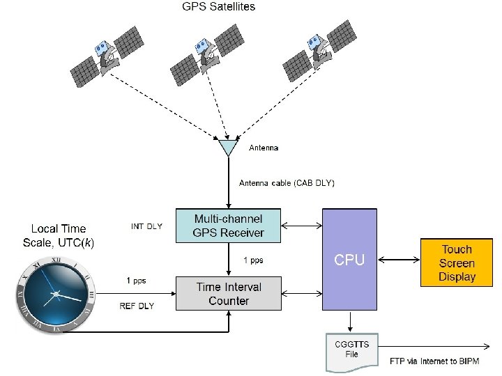
GPS Satellites Common-view GPS data is normally post processed, but it can be processed in real time with the help of the Internet. This is the method used by the SIM Time Network. Clock B Clock A GPS Receiver Time Interval Counter Internet Server for real-time processing Time Interval Counter Clock B – Satellite(s) Clock A – Satellite(s) Web site showing results of Clock A – Clock B

The SIM Time Network

The SIM Time Network ü The SIM Time Network is a common-view GPS network that processes its data in realtime. All participants use identical measurement equipment. ü Data can be processed as common-view or all-in-view measurements. ü A total of 25 national metrology institutes laboratories now have the SIM equipment, and 23 have at least periodically contributed to the network. Eleven now have cesium clocks and contribute to the SIM Time Scale (SIMT).

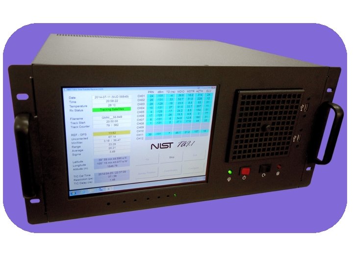
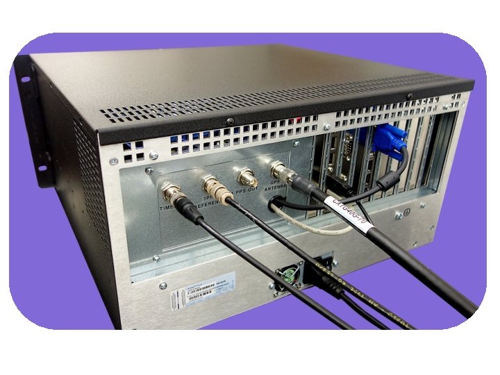
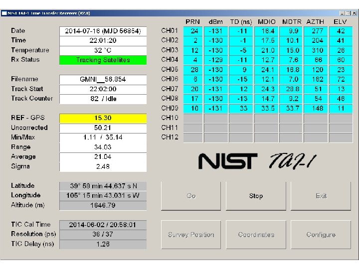
The SIM Measurement System • Simple design makes it easy and inexpensive for SIM labs to compare their clocks. It includes: ü ü 8 -channel GPS receiver (C/A code, L 1 band) Time interval counter with 30 ps resolution Rack-mount PC and flat panel display Pinwheel type antenna • The receiver measures all visible satellites and stores 1 -minute and 10 -minute REFGPS averages. • All systems are connected to the Internet, and send their files to three web servers (in Canada, Mexico, and the U. S. ) every 10 minutes. • The web server processes data “on the fly” in near real-time. Results can be viewed on the web in either common-view or all-in-view format. • All units are built and calibrated at NIST • Most systems are paid for by SIM and all become the property of the NMI.

SIM Receiver Calibrations SIM systems are calibrated at NIST prior to shipment. Calibrations are performed using the common-view, common-clock method. The SIM laboratory installs the same antenna cable and antenna that were used during the calibration. Calibrations last for 10 days. The time deviation (Type A uncertainty) of the calibration is less than 0. 2 ns after one day of averaging. The combined uncertainty is estimated at 4 ns, because a variety of factors can introduce a systematic offset.

tf. nist. gov/sim

Viewing SIMTN Measurement Results • Measurement results are displayed in HTML 5 format, and can be viewed with any web device including smartphones and tablets, with new data every 10 minutes. Users can ü Plot the time and frequency difference between SIM laboratories using the common-view method (data are averaged across all satellites and are also shown for each individual satellite). ü Display the Allan deviation and time deviation for all comparisons. ü Display 10 minute, 1 hour, and 1 day averages in tabular form. ü Plot up to 200 days of data at once. ü Process data using either “classic” common-view or all-in-view.

The SIMTN “grid” is produced by servers at CENAM, NIST, and NRC and updated every 10 minutes

Uncertainty of SIMTN Comparisons

Common-view GPS uncertainty is related to one-way uncertainty but not quite the same ü Anything that is different between the two time transfer systems involved in the comparison will add to the measurement uncertainty. However, the uncertainty is the difference between the two systems because GPS “falls out” of the common-view equation. It is possible for both systems to be in error by the same amount and for the error to be cancelled. ü Consider a situation where two systems each utilize the modelled ionospheric delay correction, and each has an average daily uncertainty of 3 ns for UBI. In this case, the uncertainty will of the ionospheric delay will cancel and be near 0. For this reason, common-view comparisons over a short baseline will remove the ionospheric delay in a similar fashion to a dual-frequency receiver.

SIM Time Network Uncertainty Analysis Uncertainty Component Best Case Worst Case Typical UA, TDEV, τ = 1 d 0. 7 5 2 UB, Calibration 1 4 2 UB, Coordinates 1 25 3 UB, Environment 2. 5 4 3 UB, Multipath 1. 5 5 2 UB, Ionosphere 1 3. 5 2 UB, Ref. Delay 0. 5 2 1 UB, Resolution 0. 05 UC, k = 2 7. 0 53. 8 11. 8 ü Uncertainties are expressed using a method complaint with the ISO GUM standard. ü Combined standard uncertainty (k = 2) is usually < 15 nanoseconds for time, and usually < 1 10 -13 for frequency after 1 day of averaging.
 by participating in the BIPM Key Comparisons")
Contributing to Coordinated Universal Time (UTC) by participating in the BIPM Key Comparisons
 n Published monthly, it contains the results of")
BIPM Circular T (www. bipm. org) n Published monthly, it contains the results of the BIPM key comparisons. Results are two to six weeks old at the time of publication. n PTB in Germany is the pivot laboratory for all comparisons. n About 70 laboratories now appear on the Circular T and contribute data to Coordinated Universal Time (UTC). n New “Rapid” UTC (UTCr) document is published every week.

Steps required in order to appear on the BIPM Circular T and contribute to UTC ü You must have a cesium clock ü You must have a CGGTTS* compatible GPS receiver (SIM system is not compatible) or the ability to submit a RINEX file. ü Your country must be a signatory of the CIPM MRA ü You must contact the BIPM and provide information on the name/address of the laboratory, clocks (model, serial number), time transfer equipment in the laboratory, and any other relevant information. They will then assign an acronym and a code to your laboratory, and a code to each clock. ü You must submit a data file once per week by FTP n * Consultative GPS and GLONASS Time Transfer Sub-committee
 on the reference date")
CGGTTS Data Collection Schedule § Starting at 0: 00 (UTC) on the reference date (October 1, 1997), the 24 hours of a day are divided into 90 16 -minute intervals. § The first 89 intervals are used for common-view. Start time of each 16 -minute interval is shifted 4 minutes earlier everyday. The 90 th interval is reserved for handling the 4 -minute start time update. § The 13 -minute common-view measurement starts 2 minutes after the beginning of the 16 -minute interval. lock up 2 1 2 3 4 0: 00 0: 16 0: 32 0: 48 measurement 13 data processing 1 90 89 1 2 23: 28 23: 44 23: 56 0: 12 1: 04 Day 1 t 0: 28 Day 2

The CGGTTS Common-view Data Format GGTTS GPS DATA FORMAT VERSION = 01 REV DATE = 11/20/2013 RCVR = NIST TAI-1 Time Transfer Receiver CH = 12 IMS = 99999 LAB = NIST X = -1288331. 833 m Y = -4721664. 612 m Z = 4078681. 021 m FRAME = WGS 84 COMMENTS = Lab Code - 10002, UTC Code - 0010002 COMMENTS = INT DLY = 25. 5 CAB DLY = 119. 8 REF DLY = 782. 4 REF = UTC(NIST) CKSUM = 07 PRN CL MJD STTIME TRKL ELV AZTH REFSV SRSV REFGPS SRGPS DSG IOE MDTR SMDT MDIO SMDI CK hhmmss s . 1 dg . 1 ns . 1 ps/s. 1 ns . 1 ns. 1 ps/s 02 FF 56842 001400 780 807 2428 -5049146 -47 201 -112 14 65 68 -1 137 -5 E 9 04 FF 56842 001400 780 349 0500 -76293 0 113 50 31 4 116 22 195 19 81 05 FF 56842 001400 780 198 1696 3610220 -26 180 -218 23 88 198 -67 33 06 FF 56842 001400 780 580 0460 -24402 37 132 -61 11 56 79 7 147 7 8 A 10 FF 56842 001400 780 410 1160 1325608 2 279 -156 22 28 101 -8 194 -20 CF 12 FF 56842 001400 780 630 3045 -2159513 -43 157 -98 11 18 75 -4 145 -8 DE 17 FF 56842 001400 780 178 0850 1062788 45 174 42 31 95 217 59 281 27 E 7 24 FF 56842 001400 780 2318 314713 1 101 -5 23 92 169 39 311 42 91 25 FF 56842 001400 780 256 3150 -247955 0 111 -72 23 108 153 -37 240 -30 E 0 02 FF 56842 003000 780 850 3044 -5049183 -57 239 120 13 65 67 0 132 -3 C 8 04 FF 56842 003000 780 281 0510 -76293 0 192 138 20 4 140 30 212 18 88

Low-Cost CGGTTS Receiver is available n A CGGTTS receiver is available through the SIM TFMWG: ü Designed at NIST, this low-cost receiver is a L 1 band only device (12 channels). Easy to use, it has a touch screen interface. ü The part number is NIST Standard Reference Instrument 60004. ü The cost is about $10, 000 USD (but is sometimes covered by SIM/OAS donations). ü It is compatible with both UTC and Rapid UTC requirements, and like the SIM system, automatically uploads data. ü Three of these units are now operating at SIM labs and contributing to UTC (Argentina, Peru, and Colombia). Other units have been shipped to Uruguay, Costa Rica, and Bolivia.

More Advanced Time Transfer Receivers More advanced time transfer receivers for UTC contributions are commercially-available, and at use at laboratories such as NRC, CENAM, and ONRJ. These receivers are dual frequency (GPS L 1 and L 2) and sometimes even receive other GNSS satellites (such as GLONASS and Galileo). They are more stable than the L 1 only receivers, and have the advantage of being able to survey their antenna more accurately, and can measure the ionospheric delay. Stefania Romisch from NIST will be demonstrating one of these receivers on Wednesday.

Other GNSS Systems
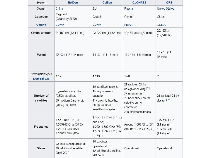

Summary ü GPS is the primary system for distributing accurate time around the world, but other GNSS systems now offer similar capability. Commonview GPS is a powerful tool for comparing remote clocks located anywhere on Earth. ü Comparing your national time standard to the standards of other countries via satellite time transfer is essential for ensuring the integrity of your measurements and for establishing international traceability. ü All SIM labs are encouraged to participate in the SIM Time Network for real-time verification of their clocks. It is very useful tool that always lets you know if your time scale is working properly. ü More established SIM labs with cesium clocks or hydrogen masers are encouraged to participate in the BIPM key comparison and to contribute to UTC.
- Slides: 70