The Global Positioning System GPS and CommonView Time
 and Common-View Time Transfer Michael Lombardi NIST Time and")
The Global Positioning System (GPS) and Common-View Time Transfer Michael Lombardi NIST Time and Frequency Division SIM Time and Frequency Metrology Working Group Workshop and Planning Meeting Panama City, Panama January 27 -29, 2015

Outline • What is GPS? • How does GPS work? • What is the uncertainty of GPS positioning? • What is the uncertainty of GPS time? • Common-view GPS time transfer • The SIM Time Network • The uncertainty of SIMTN comparisons • Contributing to UTC by participating in the BIPM key comparisons

What is GPS?
 is not only a positioning and navigation")
§ § The Global Positioning System (GPS) is not only a positioning and navigation system, but the main system used to distribute accurate time and frequency worldwide The constellation includes a maximum of 32 operational satellites § The satellites are in semisynchronous orbit at an altitude of about 20, 200 km § The orbital period is 11 hours, 58 minutes § At least four satellites, but typically seven or more, can always be received at a given location, so the entire Earth has continuous GPS coverage § The satellites carry either cesium or rubidium atomic clocks What is GPS?
 there are 31 operational GPS satellites occupying all")
GPS Satellites • Currently (January 2015) there are 31 operational GPS satellites occupying all but one of the 32 possible “slots” ü Only two satellites (PRN 10 and PRN 24) are referenced to cesium clocks, the other 29 are referenced to rubidium clocks. ü The oldest satellite is PRN 32, launched in November 1990, this was a Block IIA satellite built by Rockwell. ü The newest satellite is PRN 03, launched on October 29, 2014, a Block IIF satellite built by Boeing. Block IIR/IIR-M Built by Lockheed Martin Launched from 1997 to 2009 Block II/IIA Vehicles

GPS Control Segment n The GPS control segment includes a master control station in Colorado, an alternate master control station in California, 12 command control sites, and 16 monitoring sites that u Monitor the GPS satellites for operational health u Upload satellite almanacs, ephemeris messages, and clock corrections

How Does GPS Work?

GPS GPSSignal. Structure Two L-band carrier frequencies L 1 = 1575. 42 MHz L 2 = 1227. 60 MHz • Two PRN Codes – P(Y): Military Code ü 267 day repeat interval ü Encrypted – code sequence not published ü Available on L 1 and L 2 – C/A: Coarse Acquisition (Civilian) Code ü 1 millisecond repeat interval ü Available to all users, but only on L 1 • Code modulated with Navigation Message Data – Provides ephemeris data and clock corrections for the GPS satellites – Low data rate (50 bits per second)

GPS Modulation ü The GPS carriers are sine waves. Two binary codes are modulated onto them: the C/A (coarse/acquisition) code and the P (precise) code. ü Binary biphase modulation (also known as binary phase shift keying [BPSK]) is the technique used to modulate the codes onto the carrier. There is a 180 degree carrier phase shift each time the code state changes. ü GPS spreads the data over a bandwidth much wider than needed to carry the small amount of information. This allows very low power signals to be used. This “spread spectrum” technique is the same principle used by household cordless telephones and other devices.
![GPS Signal (L 1 band, C/A Code) P[d. BW] 2. 046 MHz C/A-CODE P-CODE](http://slidetodoc.com/presentation_image_h2/d97b8922b790e0c8fdbf34e9802e999a/image-10.jpg "GPS Signal (L 1 band, C/A Code) P[d. BW] 2. 046 MHz C/A-CODE P-CODE")
GPS Signal (L 1 band, C/A Code) P[d. BW] 2. 046 MHz C/A-CODE P-CODE -160 -163 1575. 42 MHz P[d. BW] f [Hz] L 1 Signal 20. 46 MHz Frequency Spectrum n C/A stands for Coarse Acquisition. The C/A code, broadcast on the L 1 carrier at 1575. 42 MHz, is the reference for nearly all GPS consumer products, including the receivers used in the SIM Time Network. n The C/A code is freely available to anyone, worldwide, as part of the Standard Positioning Service (SPS) of GPS.
")
GPS L 1 C/A Signal (Time-Domain)

GPS Positioning • GPS positioning is based on: ü The precise measurement of time ü The constancy of the speed of light • GPS positioning uses the concept of trilateration ü GPS satellite positions are known ü Receiver position is not known ü GPS-to-receiver range measurements are used to compute position

Positioning Example with One Transmitter Locus of points on which the receiver can be located Receiver (location unknown) Measured Range Transmitter (location known)

Positioning Example with Two Transmitters True Receiver Location r 1 T 1 r 2 T 2 False Receiver Location

Positioning Example with Three Transmitters True Receiver Location r 1 T 1 r 3 r 2 T 3

Solving for Receiver Position and Time • The position solution involves solving for four unknowns: ü Receiver position (x, y, z coordinates) ü Time • A positioning uncertainty of about 10 meters requires the time of the receiver clock to be known to within about 30 ns, because the speed of light is about 3 ns per meter. • The solution requires: ü Range measurements to each satellite to determine the signal propagation delay ü Reading the data message from each satellite to obtain the satellite’s location and corrections for the satellite clock
 Codes ü Each GPS satellite transmits own unique Pseudo-Random Noise (PRN)")
Pseudo-Random Noise (PRN) Codes ü Each GPS satellite transmits own unique Pseudo-Random Noise (PRN) Code. There are 32 possible codes (PRN 1 to 32), one for each satellite in the constellation. ü The C/A Code repeats every millisecond. ü Remember, all satellites broadcast on the same frequency (1575. 42 MHz in the case of L 1). The receiver can only distinguish between satellites by generating replicas of the C/A code and using code correlation to “get a lock. ”

Locking to a Satellite by Matching the C/A Code GPS transmitted C/A code Receiver replicated C/A code Dt Finding ∆t for each GPS signal tracked is called “code correlation”. The receiver locks to the satellite by matching the code it generates to the code transmitted by the satellite. ü Once the receiver has locked to a satellite, it can make a range measurement ü Dt is proportional to the GPS-to-receiver range (the propagation delay).
 --Satellite PRN sequence Receiver PRN sequence")
Ranging Measurements ( xs, ys, zs, ts ) --Satellite PRN sequence Receiver PRN sequence ( x, y, z, t ) pr Receiver pseudo-range --- [s] [m]

The range measurement produces not the true geometric range, but rather the pseudorange. Errors are introduced by the satellite clock and receiver clock errors (primarily by the receiver clock), by delays as the signals pass through the ionosphere and troposphere, and by multipath and receiver/antenna noise. The pseudorange equation is p = ρ + c × (dt − d. T ) + dion + dtrop + rn where ü p is the pseudorange ü c is the speed of light ü ρ is the geometric range to the satellite ü dt and d. T are the time offsets of the satellite and receiver clocks with respect to GPS time ü dion is the delay through the ionosphere (an estimate can be obtained from the GPS broadcast) ü dtrop is the delay through the troposphere ü rn represents the effects of receiver and antenna noise, including multipath.

What is the uncertainty of GPS positioning?

Factors that Limit the Uncertainty of GPS Positioning • Two main factors limit the uncertainty of the GPS positioning solution ü UERE (User Equivalent Range Error) ü Reflects the uncertainty of the pseudo range measurements between a particular satellite and the receiver ü DOP (Dilution of Precision)
 (URE), meters RMS Signal-in-Space User Range UERE accuracy exceeds")
RMS SIS URE Error (m) (URE), meters RMS Signal-in-Space User Range UERE accuracy exceeds published standard 7 N/A N/A N/A Signal-in-Space User Range Error is the difference between a GPS satellite’s navigation data (position and clock) and the truth, projected on the lineof-sight to the user 2001 SPS Performance Standard (RMS over all SPS SIS URE) 6 5 2008 SPS Performance Standard (Worst of any SPS SIS URE) 4 3 2 1. 6 Decrea sing ra nge err or 1. 2 1. 1 2004 2006 1 1. 0 0. 9 2008 2009 0 1992 1994 1996 Selective Availability (SA) 1997 2001
 ü Depends upon the geometry of satellites, as seen by")
Dilution of Precision (DOP) ü Depends upon the geometry of satellites, as seen by the receiver. ü If the satellites used in the positioning solution are spread out in the sky, the DOP is lower and the position estimate has less uncertainty. Good (Low) DOP Conditions: Poor (High) DOP Conditions:

GPS Positioning Accuracy Specifications U. S. commitments to civil GPS performance are documented in the GPS Standard Positioning Service Performance Standard (2008). ü With averaging, the horizontal uncertainty (latitude and longitude) can often be reduced to less than one meter. It should be less than 10 meters with no averaging. ü The vertical uncertainty (altitude) does not improve significantly with averaging, and can be greater than 10 meters.

What is the uncertainty of GPS time?

GPS can be trusted as a reference for measuring position, distance, and time • GPS requires highly accurate timing derived from atomic clocks, or the navigation system will fail – Assume that the maximum acceptable uncertainty contribution from the GPS clocks is 1 m: ü Light travels 3 x 10⁸ m/s, thus a 1 m error equals a 3. 3 ns timing uncertainty ü The clocks must be stable enough to keep time to better than 3. 3 ns for 12 hours, the approximate period between clock corrections ü This requires better than 1 x 10 -13 stability (3. 3 x 10 -9 s / 43200 s = 0. 8 x 10 -13) • The atomic oscillators onboard the satellites are steered from U. S. Air Force ground stations to agree with the Coordinated Universal Time (UTC) time scale maintained by the U. S. Naval Observatory, known as UTC(USNO).
,")
GPS time is a very close approximation of UTC ü Coordinated Universal Time (UTC), computed monthly by the Bureau International des Poids et Mesures (BIPM), is the official world time scale. ü UTC(USNO) is a real time approximation of UTC that is nearly always within 10 ns of UTC (0. 01 µs). ü Subframe 4 of the GPS navigation message includes a UTC(USNO) time difference correction. This correction is applied by default by GPS timing receivers (most receivers do not even allow the corrections to be turned off). ü UTC(USNO) is the time scale distributed by GPS receivers.
, Circular-T, 2008 -2012 foff = 0. 9 × 10 -17")
UTC – UTC(USNO), Circular-T, 2008 -2012 foff = 0. 9 × 10 -17
, Circular-T, 2008 -2012 foff = 4. 5 × 10 -17")
UTC – UTC(NIST), Circular-T, 2008 -2012 foff = 4. 5 × 10 -17
 – UTC(USNO), Circular-T, 2008 -2012 foff = -3. 6 × 10 -17")
UTC(NIST) – UTC(USNO), Circular-T, 2008 -2012 foff = -3. 6 × 10 -17
 – UTC(USNO), via GPS Rx in SIM System, 2008 -2012 foff = -1.")
UTC(NIST) – UTC(USNO), via GPS Rx in SIM System, 2008 -2012 foff = -1. 4 × 10 -17

Common-View GPS Time Transfer

“Classic” Common-View GPS Measurements Common-view GPS is the most practical and cost effective way to compare two clocks at remote locations. The common-view method involves a GPS satellite (S) that can be received at each of two receiving sites (A and B). Each site has a GPS receiver, a clock, and a time interval counter. The time interval between the local clock and GPS is measured at each site. Two data sets are recorded (one at each site): ü ü Clock A - S Clock B - S The two data sets are then subtracted from each other to find the difference between Clocks A and B. Delays that are common to both paths (d. SA and d. SB) cancel. Delays that are not common to both paths contribute uncertainty to the measurement. The equation for the measurement is: (Clock A – S) – (Clock B – S) = (Clock A – Clock B) + (d. SA – d. SB)

All-in-view GPS § Instead of requiring the same individual satellite to be received at both locations, this method takes the average of all of the satellites that can be received, and then measures the time difference between the group of satellites and the local clock. § As is the case with classic common-view, the two measurements are then subtracted from each other to obtain the difference between two clocks. § This method works over very long baselines when no satellites are in common-view. For example, it allows continuous comparisons between Brazil and Canada, or Brazil and the United States. In fact, it allows commonview systems to be located anywhere on Earth. § The performance is perhaps a little worse than classic common-view for short baselines (2500 km or less), but better than classic common-view for long baselines (5000 km or longer) A B

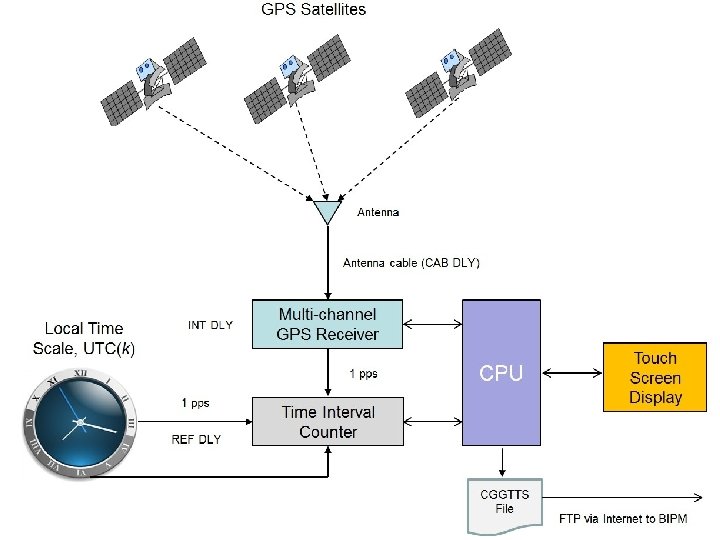
GPS Satellites Common-view GPS data is normally post processed, but it can be processed in real time with the help of the Internet. Clock B Clock A GPS Receiver Time Interval Counter Internet Server for real-time processing Time Interval Counter Clock B – Satellite(s) Clock A – Satellite(s) Web site showing results of Clock A – Clock B

A few things to know about common-view ü Common-view systems need to be calibrated so that the difference in delays between two systems is as close to 0 as possible. ü Anything that is different between two common-view systems will add to the measurement uncertainty. For example, if the antenna coordinates are wrong at one site, it will add uncertainty to the clock comparison. ü GPS time is not the reference! Common-view is a way to compare clocks to each other, for example to compare the clock at NIST to the clock at CENAMEP. GPS is simply used as a transfer standard to compare clocks located at remote sites. Even if the GPS time were wrong, it would not affect the common-view comparison.

The SIM Time Network
 recognized")
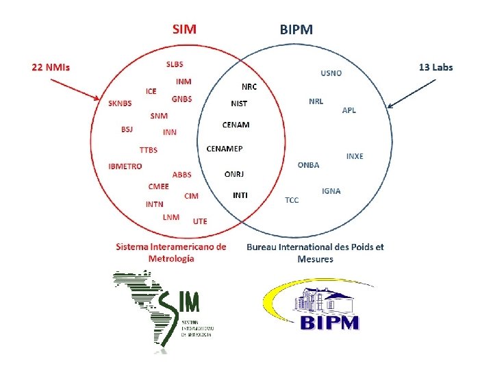
Information about SIM ü SIM is one of five regional metrology organizations (RMOs) recognized by the BIPM. ü The BIPM expects RMOs to review the quality systems of NMIs, and their calibration and measurement capabilities (CMCs). RMOs should also organize regional comparisons to supplement the BIPM key comparisons so that more nations can establish traceability to the SI. This is the role of the SIMTN. ü SIM consists of NMIs located in the 34 member nations of the Organization of American States (OAS), which extends throughout North, Central, and South America, and the Caribbean region. ü SIM is the largest RMO in terms of land area, and the SIM region now has almost one billion people. About 2 out of 3 people in the SIM region live in the United States, Brazil, or Mexico. ü SIM has organized metrology working groups (MWGs) in 11 different areas, including time and frequency. The SIM Time Network is operated by the T&F MWG.

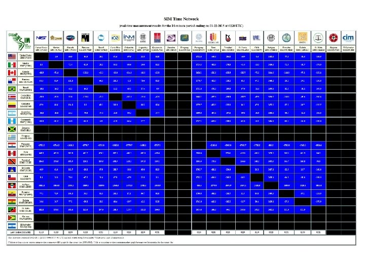
The SIM Time Network ü The SIM Time Network is based on real-time commonview GPS comparisons. All participants use identical measurement equipment. ü Data can be processed as common-view or all-in-view measurements. ü A total of 22 laboratories now participate, with two nations currently on the waiting list as of January 2015. All of these labs continuously compare their clocks, 24 hours per day, 7 days per week.
 Clock Group United States")
Country Organization Year of First Participation Time Standard (SIMT clock) Clock Group United States NIST 2005 Ensemble time scale 1 Mexico CENAM 2005 Ensemble time scale 1 Canada NRC 2005 Ensemble time scale 1 Panama CENAMEP 2005 Cesium clock 2 Brazil ONRJ 2006 Ensemble time scale 1 Costa Rica ICE 2007 Cesium clock 2 Colombia INM 2007 Cesium clock 2 Argentina INTI 2007 Cesium clock 2 Guatemala LNM 2007 GPS disciplined clock 3 Jamaica BSJ 2007 Cesium clock 2 Uruguay UTE 2008 Cesium clock 2 Paraguay INTN 2008 SIMT disciplined rubidium clock 4 Peru INDECOPI 2009 Cesium clock 2 Trinidad & Tobago TTBS 2009 GPS disciplined clock 3 Saint Lucia SLBS 2010 SIMT disciplined rubidium clock 4 Chile INN 2010 SIMT disciplined rubidium clock 4 Antigua and Barbuda ABBS 2011 SIMT disciplined rubidium clock 4 Ecuador CMEE 2012 GPS disciplined clock 3 Bolivia IBMETRO 2012 SIMT disciplined rubidium clock 4 St. Kitts and Nevis SKNBS 2014 SIMT disciplined rubidium clock 4 Guyana GNBS 2015 SIMT disciplined rubidium clock 4 El Salvador CIM 2015 SIMT disciplined rubidium clock 4 Dominican Republic INDOCAL 2015? SIMT disciplined rubidium clock 4 Belize BBS 2015? SIMT disciplined rubidium clock 4

SIM Time Network Design Goals n Our design goals were: ü To establish cooperation and communication between the SIM time and frequency labs now and in the future. ü To build a network that allowed all SIM NMIs to compare their time standards to those of the rest of the world. ü To utilize equipment that was low cost and easy to install, operate, and use, because SIM NMIs typically have small staffs and limited resources. ü To be capable of measuring the best standards in the SIM region. This meant that the measurement uncertainties had to be as small, or nearly as small, as those of the BIPM key comparisons. ü To report measurement results in near real-time, without the processing delays of the BIPM key comparisons. ü To build a democratic network that favored no single laboratory or nation, and to allow all members to view the results of all comparisons.

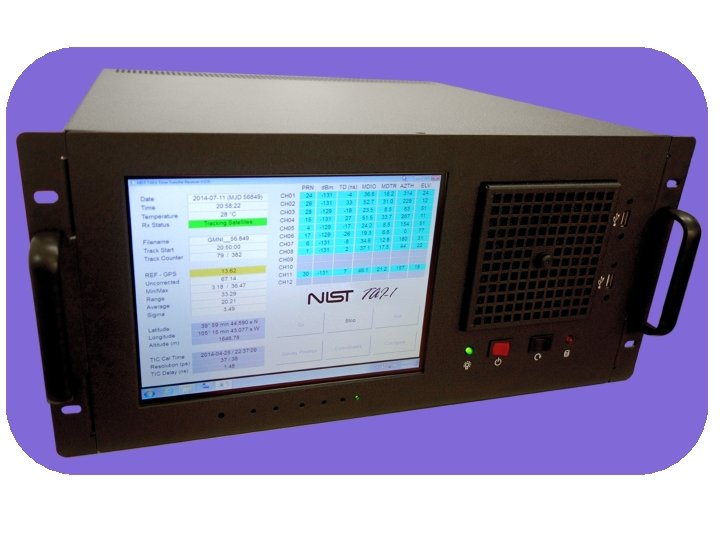
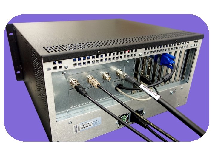
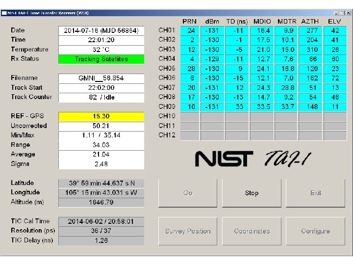
The SIM Measurement System • Simple design makes it easy and inexpensive for SIM labs to compare their clocks. It includes: ü ü 8 -channel GPS receiver (C/A code, L 1 band) Time interval counter with 30 ps resolution Rack-mount PC and flat panel display Pinwheel type antenna • The receiver measures all visible satellites and stores 1 -minute and 10 -minute REFGPS averages. • All systems are connected to the Internet, and send their files to three web servers (in Canada, Mexico, and the U. S. ) every 10 minutes. • The web server processes data “on the fly” in near real-time. Results can be viewed on the web in either common-view or all-in-view format. • All units are built and calibrated at NIST • Most systems are paid for by SIM and become the property of the NMI.

tf. nist. gov/sim
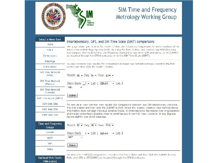

Viewing SIMTN Measurement Results • Measurement results can be viewed with any web device, with new data every 10 minutes. Users can ü Plot the time and frequency difference between SIM laboratories using the common-view method (data are averaged across all satellites and are also shown for each individual satellite). ü Display the Allan deviation and time deviation for all comparisons. ü Display 10 minute, 1 hour, and 1 day averages in tabular form. ü Plot up to 200 days of data at once. ü Process data using either “classic” common-view or all-in-view.

HTML 5 displays work on smartphones and tablets

Uncertainty of SIMTN Comparisons

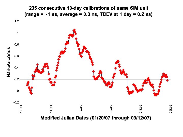
SIM Receiver Calibrations SIM systems are calibrated at NIST prior to shipment. Calibrations are performed using the common-view, common-clock method. The SIM laboratory installs the same antenna cable and antenna that were used during the calibration. Calibrations last for 10 days. The time deviation (Type A uncertainty) of the calibration is less than 0. 2 ns after one day of averaging. The combined uncertainty is estimated at 4 ns, because a variety of factors can introduce a systematic offset.

Uncertainty due to Antenna Coordinates n GPS computes dimensions in Earth-Centered, Earth-Fixed X, Y, and Z coordinates that the receiver converts to geodetic latitude, longitude, and altitude. ü Coordinate errors translate to timing errors, typically about 2. 2 ns per meter for a multichannel receiver. ü The SIM system has a built-in antenna survey feature that can determine horizontal position (latitude/longitude) to within < 1 meter after 24 hours of averaging. ü However, the SIM system does a poor job of determining vertical position (altitude). There is nearly always a bias that can exceed 10 ns (a timing error of of 20 to 30 nanoseconds). ü For best results, the altitude of the SIM GPS antenna should be independently surveyed, or checked using a dual frequency receiver.

Average position error of repeated survey was 5. 37 m, with nearly all of this error (5. 30 m) in the vertical position

Uncertainty due to Environment ü Receiver, antenna, and cable delays can change over time due to temperature, sometimes by as much as several nanoseconds. ü GPS receivers are usually more sensitive to temperature than antennas or cables. The SIM receiver can experience a delay change of several nanoseconds if there is a sudden change in laboratory temperature. ü The SIM system uses a high quality antenna cable (LMR-400) with a low temperature coefficient. Delay changes due to temperature are usually much smaller than 1 ns, even in places like Colorado where the temperature has a very wide range over the course of a year.

Uncertainty due to Multipath n Multipath is caused by GPS signals being reflected from surfaces near the antenna. Metal objects, such as a metal roof below the antenna, are one of the worst sources of multipath reflections. The reflected signals can then either interfere with, or be mistaken for, the signals that follow the straight line path from the satellite. n If the antenna has a clear, unobstructed view of the sky, the uncertainty due to multipath is usually very small (a few nanoseconds or less). n The pinwheel type antenna used by the SIM systems also helps keep multipath to a minimum.

GPS Antennas

Uncertainty due to Ionospheric Delays ü The ionosphere is the part of the atmosphere extending from about 70 to 500 km above the earth. ü When signals from the satellites pass through the ionosphere their path is bent slightly, changing the delay. The delay changes are largest for the satellites at low elevation angles. ü GPS broadcasts a ionospheric correction, which is automatically applied by the SIM system. This reduces the effect. These corrections are called modeled ionospheric corrections, or MDIO. ü For the very best results, the ionospheric conditions are measured at a receiving location on the ground by a dual -frequency GPS receiver (one that receives both L 1 and L 2). These measurements are used in place of the broadcast corrections. This improves the results. These corrections are called measured ionosphere corrections, or MSIO. They are not applied by the SIM system, which uses the L 1 band only and cannot measure the ionospheric delay.

GPS Antennas

SIM Time Network Uncertainty Analysis Uncertainty Component Best Case Worst Case Typical UA, TDEV, τ = 1 d 0. 7 5 2 UB, Calibration 1 4 2 UB, Coordinates 1 25 3 UB, Environment 2. 5 4 3 UB, Multipath 1. 5 5 2 UB, Ionosphere 1 3. 5 2 UB, Ref. Delay 0. 5 2 1 UB, Resolution 0. 05 UC, k = 2 7. 0 53. 8 11. 8 ü Uncertainties are expressed using a method complaint with the ISO GUM standard. ü Combined standard uncertainty (k = 2) is usually < 15 nanoseconds for time, and usually < 1 10 -13 for frequency after 1 day of averaging.
 by participating in the BIPM Key Comparisons")
Contributing to Coordinated Universal Time (UTC) by participating in the BIPM Key Comparisons
 n Published monthly, it contains the results of")
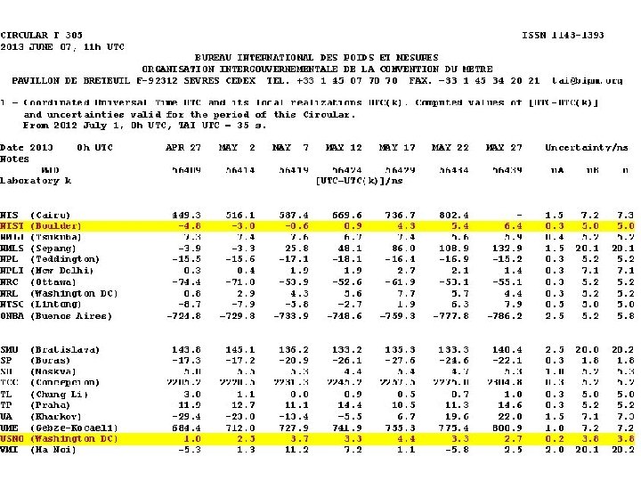
BIPM Circular T (www. bipm. org) n Published monthly, it contains the results of the BIPM key comparisons. Results are two to six weeks old at the time of publication. n PTB in Germany is the pivot laboratory for all comparisons. n About 70 laboratories now appear on the Circular T and contribute data to Coordinated Universal Time (UTC). n New “Rapid” UTC (UTCr) document is published every week.

Steps required in order to appear on the BIPM Circular T and contribute to UTC ü You must have a cesium clock ü You must have a CGGTTS* compatible GPS receiver (SIM system is not compatible) ü Your country must be a signatory of the CIPM MRA ü You must contact the BIPM and provide information on the name/address of the laboratory, clocks (model, serial number), time transfer equipment in the laboratory, and any other relevant information. They will then assign an acronym and a code to your laboratory, and a code to each clock. ü You must submit a data file once per week by FTP n * Consultative GPS and GLONASS Time Transfer Sub-committee
 on the reference date")
CGGTTS Data Collection Schedule § Starting at 0: 00 (UTC) on the reference date (October 1, 1997), the 24 hours of a day are divided into 90 16 -minute intervals. § The first 89 intervals are used for common-view. Start time of each 16 -minute interval is shifted 4 minutes earlier everyday. The 90 th interval is reserved for handling the 4 -minute start time update. § The 13 -minute common-view measurement starts 2 minutes after the beginning of the 16 -minute interval. lock up 2 1 2 3 4 0: 00 0: 16 0: 32 0: 48 measurement 13 data processing 1 90 89 1 2 23: 28 23: 44 23: 56 0: 12 1: 04 Day 1 t 0: 28 Day 2

The CGGTTS Common-view Data Format GGTTS GPS DATA FORMAT VERSION = 01 REV DATE = 11/20/2013 RCVR = NIST TAI-1 Time Transfer Receiver CH = 12 IMS = 99999 LAB = NIST X = -1288331. 833 m Y = -4721664. 612 m Z = 4078681. 021 m FRAME = WGS 84 COMMENTS = Lab Code - 10002, UTC Code - 0010002 COMMENTS = INT DLY = 25. 5 CAB DLY = 119. 8 REF DLY = 782. 4 REF = UTC(NIST) CKSUM = 07 PRN CL 02 04 05 06 10 12 17 24 25 02 04 FF FF FF MJD 56842 56842 56842 STTIME TRKL ELV AZTH hhmmss s. 1 dg 001400 780 807 2428 001400 780 349 0500 001400 780 198 1696 001400 780 580 0460 001400 780 410 1160 001400 780 630 3045 001400 780 178 0850 001400 780 2318 001400 780 256 3150 003000 780 850 3044 003000 780 281 0510 REFSV SRSV. 1 ns. 1 ps/s -5049146 -47 -76293 0 3610220 -26 -24402 37 1325608 2 -2159513 -43 1062788 45 314713 1 -247955 0 -5049183 -57 -76293 0 REFGPS SRGPS DSG IOE MDTR SMDT MDIO SMDI CK. 1 ns. 1 ps/s 201 -112 14 65 68 -1 137 -5 E 9 113 50 31 4 116 22 195 19 81 180 -218 23 88 198 -67 33 132 -61 11 56 79 7 147 7 8 A 279 -156 22 28 101 -8 194 -20 CF 157 -98 11 18 75 -4 145 -8 DE 174 42 31 95 217 59 281 27 E 7 101 -5 23 92 169 39 311 42 91 111 -72 23 108 153 -37 240 -30 E 0 239 120 13 65 67 0 132 -3 C 8 192 138 20 4 140 30 212 18 88

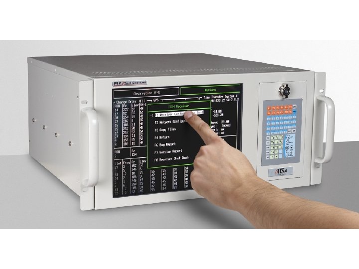
New Low-Cost CGGTTS Receiver is available now n A new CGGTTS is available through the SIM TFMWG: u Designed at NIST, this low-cost receiver is a L 1 band only device (12 channels). Easy to use, it has a touch screen interface. u The part number is NIST Standard Reference Instrument 60004. u The cost is about $10, 000 USD (but is sometimes covered by SIM/OAS donations). u It is compatible with both UTC and Rapid UTC requirements, and like the SIM system, automatically uploads data. u The first unit is operating at INTI in Argentina. Two units have been shipped recently to Colombia and Peru. Units are expected to be shipped this year to Uruguay and Costa Rica.

Other CGGTTS Time Transfer Receivers More sophisticated CGGTTS receivers are commercially-available, and at use at laboratories such as NRC, CENAM, and ONRJ. These receivers are dual frequency (GPS L 1 and L 2) and sometimes even receive other GNSS satellites (such as GLONASS and Galileo). They are more stable than the L 1 only receivers, and have the advantage of being able to survey their antenna more accurately, and can measure the ionospheric delay. However, the cost is high, sometimes as much as $40, 000 USD. Some models include: ü PIK Time TTS-4 ü Dicom GTR 50 ü Novatel

Labs in the Americas that Contribute to UTC Laboratory Country NMI or DI Time Scale UTC contributor Link to UTC Link Calibration INTI Argentina NMI Cesium Y GPS NIST ONBA Argentina DI Cesium Y GPS USNO IGNA Argentina --- Cesium Y GPS USNO ONRJ Brazil DI Ensemble Y GPS NIST INXE Brazil NMI Cesium Y GPS USNO NRC Canada NMI Ensemble Y GPS NIST TCC Chile --- Cesium Y GPS USNO CENAM Mexico NMI Ensemble Y GPS NIST CENAMEP Panama NMI Cesium Y GPS NIST United States NMI Ensemble Y TWSTFT --- USNO United States --- Ensemble Y TWSTFT --- NRL United States --- Ensemble Y GPS USNO APL United States --- Ensemble Y GPS USNO INM Colombia NMI Cesium N* GPS* NIST ICE Costa Rica DI Cesium N* GPS* NIST SNM Peru NMI Cesium N* GPS* NIST UTE Uruguay NMI Cesium N* GPS* NIST * expected to begin UTC contributions in 2015

Summary ü Common-view GPS is a powerful tool for comparing remote clocks located anywhere on Earth. ü Participation in international comparisons – comparing your national time standard to the standard in other countries – is essential for ensuring the integrity of your measurements and for establishing international traceability. ü All SIM labs are encouraged to participate in the SIM Time Network for real-time verification of their clocks. ü More established SIM labs are encouraged to participated in the BIPM key comparison and to contribute to UTC.
- Slides: 75