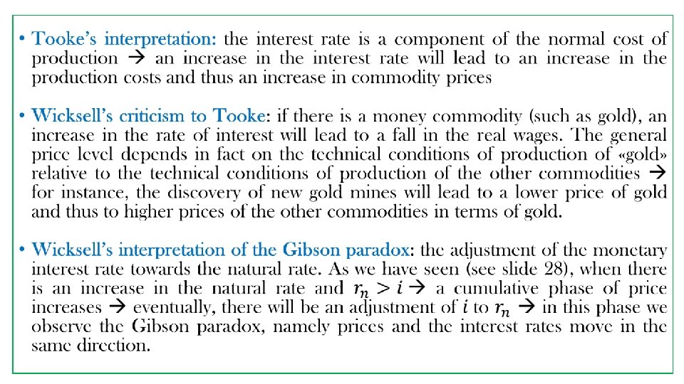
The Gibson Paradox We mentioned above the Gibson

The Gibson Paradox • We mentioned above the Gibson paradox and its modern version labelled «price puzzle» that suggests a direct relation between the price level and the interest rate. • The co-movement between the long term interest rates and prices was first stressed by Tooke (1838) in his History of Prices and discussed among others by Wicksell (1898), Fisher (1911; 1930), Keynes (1930) and Friedman&Schwartz (1976; 1982). It was labelled a paradox by Keynes in the Treatise on Money on the basis of the data provided by Gibson in a 1923 article for Banker’s Magazine. Keynes (1930, 2: 198) commented that the observed correlation was “one of the most completely established empirical facts in the whole field of quantitative economics”. Fisher (1930: 399) on the other hand observed that “no problem in economics has been more hotly debated” and Friedman&Schwartz (1976: 288) concluded that “the Gibsonian Paradox remains an empirical phenomenon without a theoretical explanation”. It is labelled a paradox because it is usually stated that a fall in the interest rate would lead to an an increase in prices and output. • Note that the co-movement does not concern the nominal rate of interest and the rate of price inflation, namely it does not refer to some kind of Fisher’s effect according to which the nominal rate of interest would adapt to changes in the expected rate of inflation. Thus Shiller and Siegel (1977) reported that movements in nominal rates in the period

The world price level and the consol yield The log of the price index and the long -term interest rate (UK)(Source: Shiller and Siegel)

• The same interpretation in terms of an adjustment in the monetary rate of interest to a previous change in the capital profitability is traceable in Fisher (1930), Keynes (1930) and Friedman&Schwartz (1976). In Fisher (1930) the phenomenon is also explained by money illusion and the fact that, due to adaptive expectations, changes in the inflation rates are not perfectly embodied in the nominal interest rates. The consequent discrepancies between the actual real interest rate and the natural rate of interest lead to fluctuations in output and prices around their trend levels. Again, the adjustment process will lead eventually to a co-movement of prices and the interest rates (see again slides 26 and 27). • However, Friedman&Schwartz (1982) and Barsky&Summers (1988) ascribe the Gibson paradox precisely to the gold standard. According to them, it manifests clearly only between 1820 -1913 but it is weak during the pre-Napoleonic period 1730 -96 and the interwar years 1921 -1938 due to the restricted functioning of the gold standard. Moreover the Gibson Paradox would be absent during the Napoleonic war period (1797 -1820) and after 1971 when the gold standard was abandoned. • According to Barsky and Summer the manifestation of the Gibson Paradox during the gold standard is due to the fact that, when there is a shock in the natural rate of interest (and thus in the rate of return of assets alternative to gold), the real price of gold change. So, if there is an increase in the rate of interest, the carrying cost of non monetary gold raises (the supply of monetary gold increases) while the demand for monetary gold falls if the demand for money is elastic to the interest rate. Therefore there is a decrease in the demand for monetary gold relative to its supply

• The existence of the Gibson paradox also in the case of a fiat money economy (namely, in the absence of the gold standard) has been restated, however, by Sims (1992) and others (for instance, Bernanke and Blinder, 1992; Christiano, Eichenbaum, and Evans, 1994). It has been renamed by Eichenbaum (1992) the «price puzzle» and assessed by models that attempt to isolate the movements in the federal funds rate that are uncorrelated with changes in the other variables in the model and, thereby, represent purely exogenous movements in the federal funds rate, or exogenous monetary policy actions (that is, shocks in the monetary policy). • The interpretations of the «price puzzle» can be distinguished into two strands. The first one explains it referring to identification problems in the estimates of the co-movement of prices and the interest rates. Sims (1992) stated that it disappears when considering also the prices of imported inputs together with the GDP deflator (in this case it is only the consequence of the reaction to a «supply shock» leading to an increase in prices by raising interest rate). Moreover, Sims explains the «price puzzle» in terms of a scant reaction of the monetary authorities to expected increases in price inflation. In this case, while the nominal rate of interest increases, the real rate of interest would not increase, and thus the increase in the nominal rate of interest is accompanied with an increase in prices. Similar interpretations were advanced by Castelnuovo and Surico (2006): the price puzzle is present when the reaction of the monetary authorities to price inflation is weak. Thus,

Considering the period 1960 -1993, an increase in the rate of interest is associated with a fall in output but a raise in the price level (Figure 2). However, this effect (see the black line in Figure 3) disappears in the years 1983 -1993 but it is present in the 1960 -79 period of an accomodative stance of the monetary policy

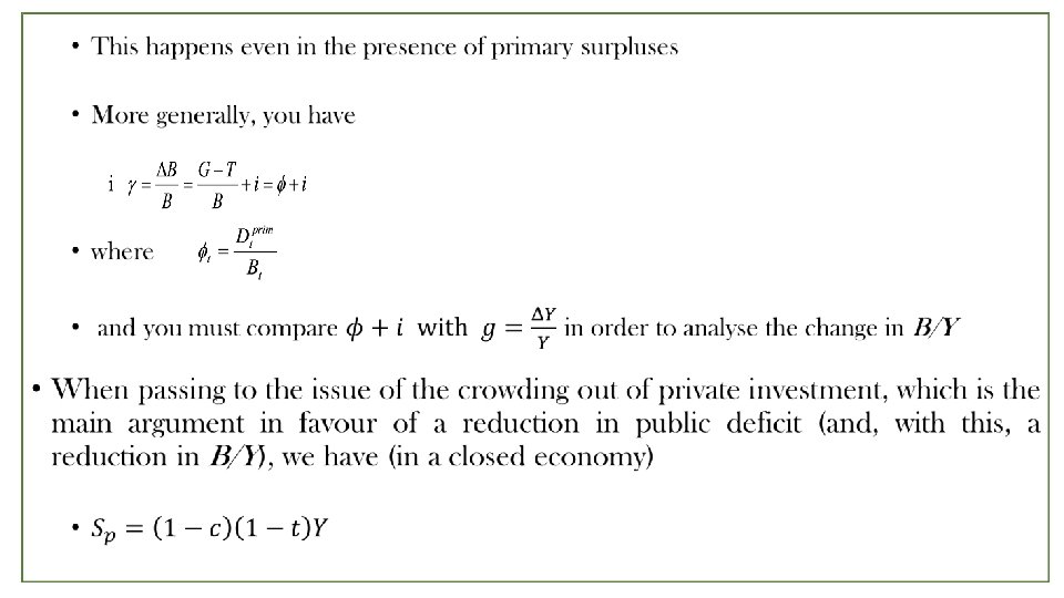
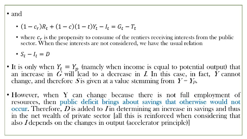
Money and public finance • When analysing monetary and fiscal policies we have considered the different ways to finance public deficits and discussed the possibility that deficit spending determines a crowding out or crowding in of private expenditure. We will now expand the analysis by addressing • a) the intertemporal public budget constraint and the debate on the sustainability of public debt; • b) the possibility to exploit monetary seigniorage to finance public deficits; • c) the different views on the effect of public deficits on growth and the public debt-income ratio according to a traditional and Keynesian approach • In order to obtain the intertemporal public budget constraint let us consider first of all the budgets of the Central Bank and of the Treasury. With respect to the Tresaury we have

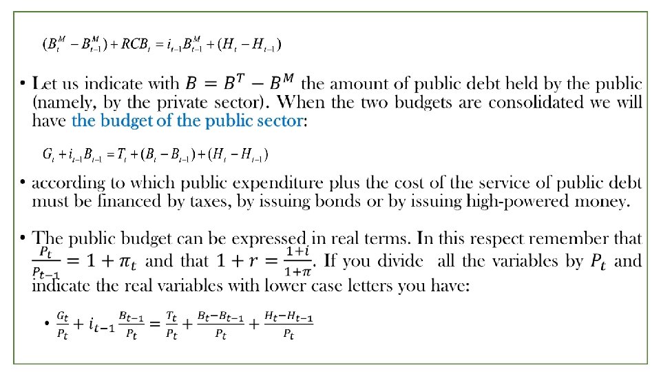
• according to which at time t the public expenditure plus the interest paid on the total stock of public debit accumulated until time t can be financed by taxes, the issuing of new bonds and the interests on the amount of public debt held by the Central Bank that are transferred to the Treasury. • [therefore, to what extent the public debt is held by the Central Bank or by the bank system is not indifferent for the Treasury: only in the first case it does not lead to a transfer to the private sector. However, CB may prefer to not hold assets in the form of public debt since a fall in the price of public bonds would determine a lower value of its assets] • When passing to the budget of the Central Bank, there is a relation that links the changes in its activities and liabilities due to its operations with the Treasury: the amount of public bonds owned by the Central Bank plus the amount of interests transferred to the Treasury must equal (can be financed by) the interests received by the Treasury for the bonds in its possession plus the change in the amount of monetary base (the issuing of high-

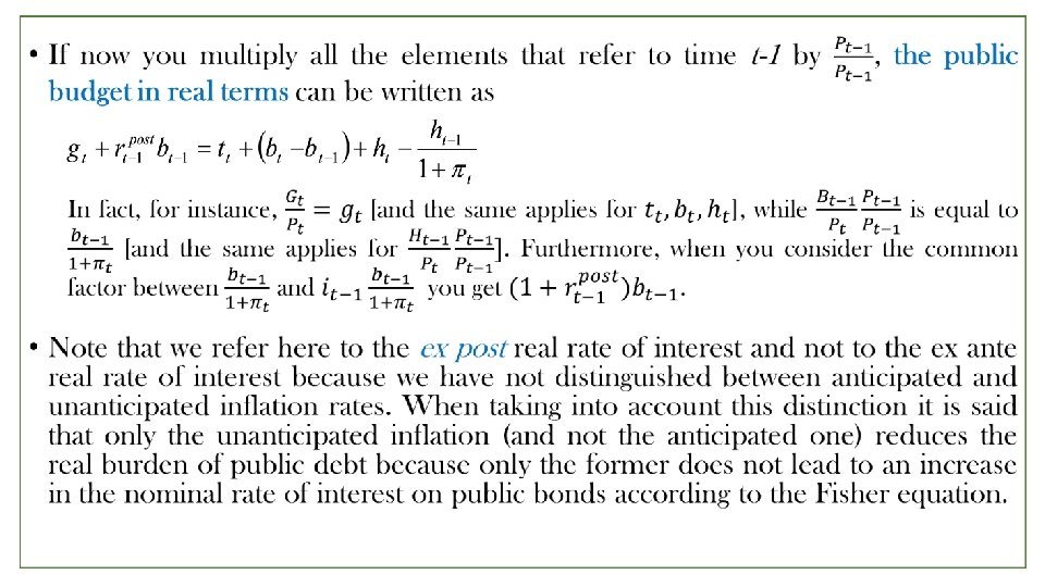
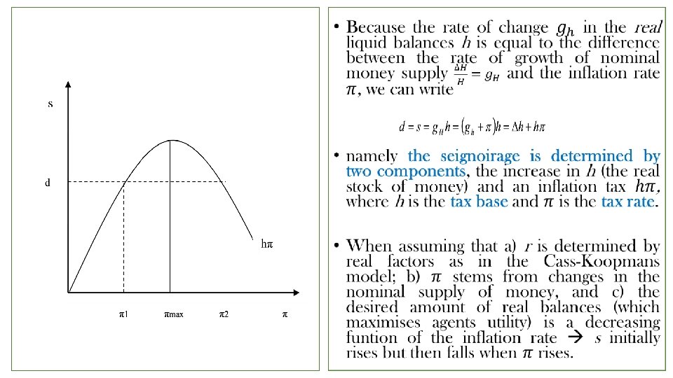
• The last two terms of the real public budget represent the seigniorage. You can also express it as • that shows that the «income» to the public sector stemming from its power to «coin» money is due to two elements: a) the change in the real liquid balances; and b) the inflation tax, which lowers the real value of the real monetary base previously issued. • Unless there are restrictions by law on the seigniorage or on borrowing from the private sector by issuing public bonds, the uniperiodal public budget constraint does not place any limits to the public sector spending. Since, however, it is believed that Governments are bound in their choices as individuals are, in order to show this bound, the intertemporal public budget constraint is advanced.

• Let us assume, for the sake of simplicity, that r is costant over time. From the uniperiodal public budget we have • and therefore • Since this holds also at time t, that is • by substituting it in the previous expression you obtain

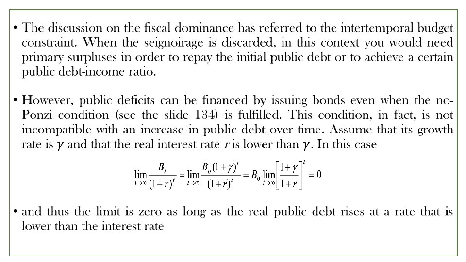
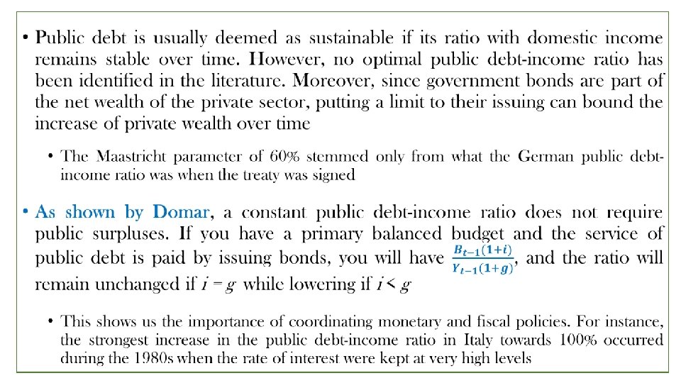
• Moreover, the intertemporal public budget constraint is not stringent when considering a time horizon that is equal to infinity because in this case you can implement primary surpluses to infinity. • Indeed, in order to discuss the sustainability of public debt, a definite time horizon is introduced. In this context, public debt becomes unsustainable when diverging from the path that would ensure the debt repayment within the assumed time period. • The idea that the public debt must be repaid or kept under control arises from • a) the extension to the State of conditions that arise for the private sector; • b) the idea that an increase in the public debt-income ratio can lead to increasing interest rates thus becoming unsustainable over time due to its continue increase; • c) the idea that public deficits determine a lower amount of private expenditure and thus that public debt substitutes other (private) forms of wealth, determining a lower capital accumulation a lower increase in labour productivity a lower increase in per capita consumption • The sustainability of public debt is analysed by referring to the public-debt income ratio due to the idea that the gross domestic product is the basis from which the amount of taxes necessary to repay public debt arises. However, two stocks should be compared (income is instead a flow variable), and very different results would occur if the public debt-private wealth ratio is

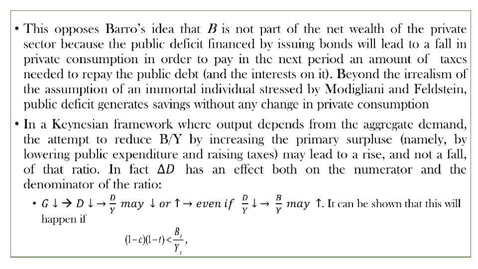
• This does not mean that public debt cannot be a problem: • Open economy the fall in the demand for government bonds when a crisis occurs the raise in the interest rates • Bounded monetary sovereignty and the power of rentiers • Portfolio effects