The Geometric Moving Average Control Chart A FullPurpose

The Geometric Moving Average Control Chart: A Full-Purpose Process-Control Tool ASQ-Baltimore Section Meeting December 10, 2002 Melvin T. Alexander Past Chair – ASQ Health Care Division

Focus: SPC Forecasting Control Chart

Outline • • • Introduction Classical vs. Modern views Comparison between charts Constructing GMA charts Example Conclusions

SPC Popular Due to • Successful in Pre-1940 s Technology • Japanese Advances in Quality • Regain Competitve Edge in 1980 s

In Catching Up We Found • Automated Systems Expanded • “Older Tools” Inadequate • Modern Tools Not Fully Used • Modern Methods Adopted/Adapted

Classical SPC “Passive” • Describes What Happened • Curative in Approach • Monitors Stability

Modern SPC “Active” • Analyzes Causes & Effect • Predicts Future • Gives Dynamic Feedback/Feedfront Basis for Action

Standard Control Chart Schemes • Shewhart • Individuals, Moving Range, & Moving Average • CUSUM • GMA (EWMA)

Shewhart Control Charts • Developed by Dr. W. A. Shewhart (1924) • Monitors Process Stability with Control Limits • Points Outside Limits Signal Instability • Places “Weight” on Latest Observation

Shewhart Charts Pros • Easy to Construct • Detects Large Process Shifts • Helps find process change caused so that countermeasures against adverse effects may be implemented

Shewhart Cons • Ignores History • Hard to Detect Small Process shifts • Hard to Predict In/Out-of. Control Processes • Really is not Process CONTROL, but is used for RESEARCH Control

Individuals, Moving Range & Moving Average Charts • Special-Case Shewhart Charts • Single Observations • Control signal Like Shewhart

Individual (I) Charts • Few Units Made • Automated Testing on Each Unit • Expensive Measurements • Slow Forming Data • Periodic (Weekly, Monthly) Adminstrative Data

Moving Range (MR) Charts • Correspond to Shewhart Range charts • Used with Individuals • Plot Absolute Differences of Successive Pairs (Lags)

Moving Average (MA) Charts • Running Average of (=4, 5) Observations • New MA Drops “Oldest” Value • Weight Places like Shewhart (n=2 for MR; n=4, 5 in MA; 0 Otherwise)

I/MA/MR Pros • Detects Small Process Shifts • Uses Limited History

I/MA/MR Cons • Auto(Serial) correlated Data Mislead Process Stability • Show Nonrandom Patterns with Random Data

Cusum Control Charts • Introduced by E. S. Page (1954) • Cumulative Sums single Observations • Points Outside V-Mask limbs • Put Equal Weight on Observations

Cusum Chart Pros • Detect “Small” Process Shifts • Uses History

Cusum Chart Cons • Fail to Diagnose Out-of-control Patterns • Hard to Construct V -Mask

Geometric (Exponetially Weighted) Moving Average (GMA/EWMA) Control Charts • Introduced by S. W. Roberts (1959) Time Series • Points Fall Outside Forecast Control Limits • Weights (w) Assign Degrees of Importance • Resembles Shewhart & Cusum Schemes

GMA(EWMA) Chart Pros • Regular Use of History • Approaches Shewhart if w=1, • Approaches Cusum if w=0

GMA (EWMA) Control chart Cons • Late in Catching Turning Points • Inaccurate for Auto(Serial) Correlated Data • Only One-ahead Forecasts Possible • Hard to Monitor Changes in Weight (w) • Allow Only One Variation Component

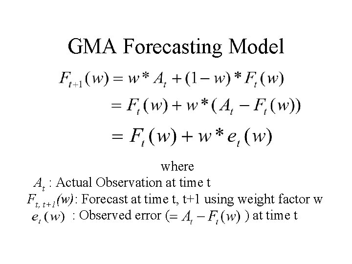
GMA Forecasting Model where At : Actual Observation at time t Ft, t+1(w): Forecast at time t, t+1 using weight factor w : Observed error ( ) at time t

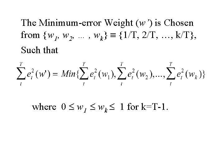
The Minimum-error Weight (w’) is Chosen from {w 1, w 2, … , wk} {1/T, 2/T, …, k/T}, Such that where 0 w 1 wk 1 for k=T-1.

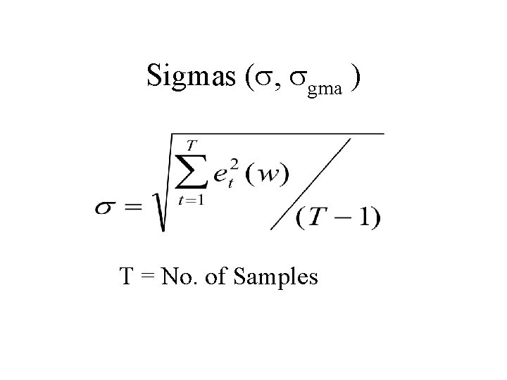
Sigmas ( , gma ) T = No. of Samples

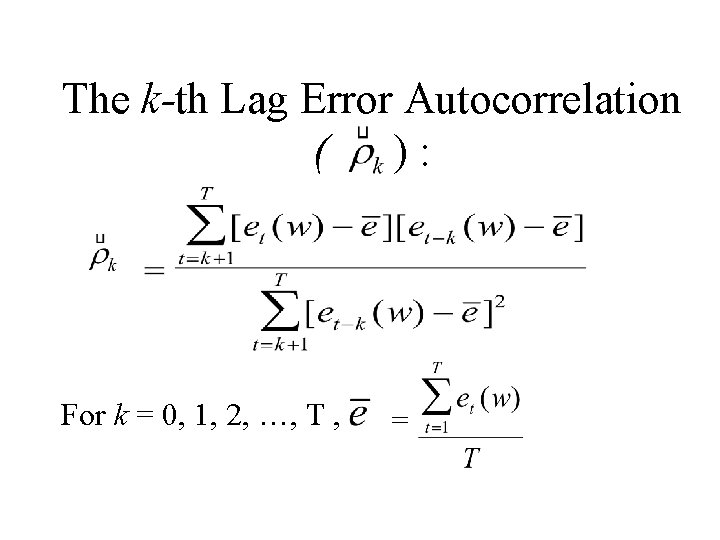
The k-th Lag Error Autocorrelation ( ): For k = 0, 1, 2, …, T , =

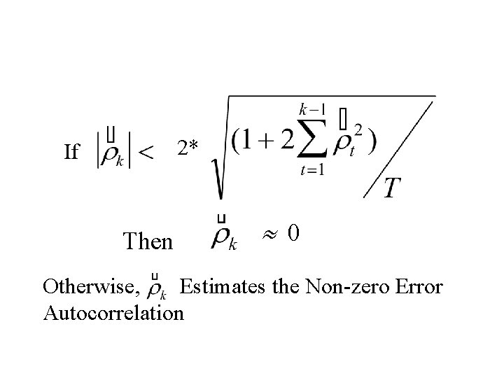
2* If Then 0 Otherwise, Estimates the Non-zero Error Autocorrelation

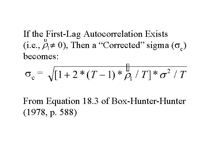
If the First-Lag Autocorrelation Exists (i. e. , 0), Then a “Corrected” sigma ( c) becomes: c = From Equation 18. 3 of Box-Hunter (1978, p. 588)

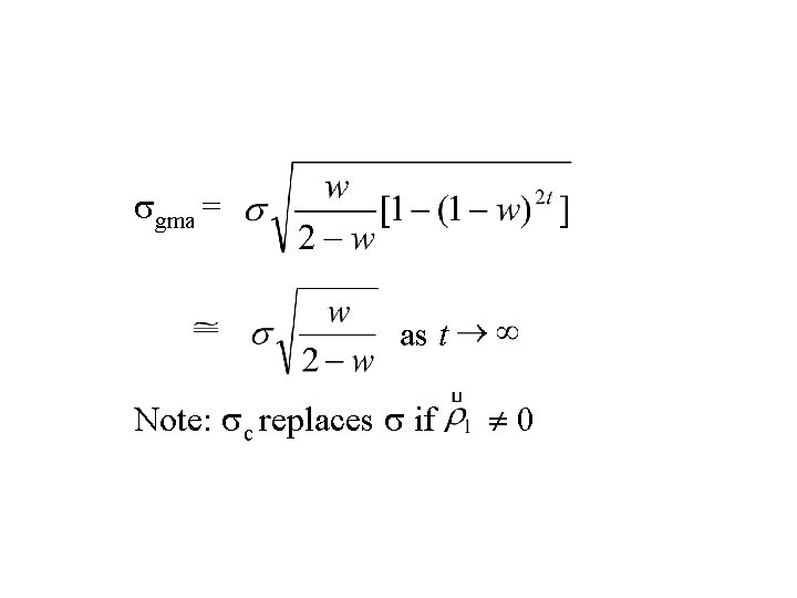
gma = as t Note: c replaces if 0

Bayes Theorem cont. Kalman filtering (Graves et al. , 2001) and Abraham and Kartha (ASQC Annual Technical Conf. Trans. , 1979) described ways to check weight stability.

Bayes Theorem cont. However, control chart plots of the errors help detect weight changes (i. e. , errors should exhibit a random pattern, if not, change the weight or the forecast method)