The explosion in hightech medical imaging nuclear medicine

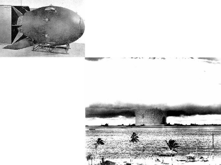
The explosion in high-tech medical imaging & nuclear medicine (including particle beam cancer treatments)

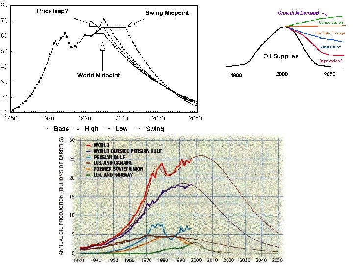
The constraints of limited/vanishing fossils fuels in the face of an exploding population

The constraints of limited/ vanishing fossils fuels …together with undeveloped or under-developed new technologies

will renew interest in nuclear power Nuclear

Fission power generators will be part of the political landscape again as well as the Holy Grail of FUSION.

…exciting developments in theoretical astrophysics The evolution of stars is well-understood in terms of stellar models incorporating known nuclear processes. The observed expansion of the universe (Hubble’s Law) lead Gamow to postulate a Big Bang which predicted the Cosmic Microwave Background Radiation as well as made very specific predictions of the relative abundance of the elements (on a galactic or universal scale).

1896 1899 1912 , g

Henri Becquerel (1852 -1908) received the 1903 Nobel Prize in Physics for the discovery of natural radioactivity. Wrapped photographic plate showed clear silhouettes, when developed, of the uranium salt samples stored atop it. 1896 While studying the photographic images of various fluorescent & phosphorescent materials, Becquerel finds potassium-uranyl sulfate spontaneously emits radiation capable of penetrating thick opaque black paper aluminum plates copper plates Exhibited by all known compounds of uranium (phosphorescent or not) and metallic uranium itself.

1898 Marie Curie discovers thorium (90 Th) Together Pierre and Marie Curie discover polonium (84 Po) and radium (88 Ra) 1899 Ernest Rutherford identifies 2 distinct kinds of rays emitted by uranium - highly ionizing, but completely absorbed by 0. 006 cm aluminum foil or a few cm of air - less ionizing, but penetrate many meters of air or up to a cm of aluminum. 1900 P. Villard finds in addition to rays, radium emits - the least ionizing, but capable of penetrating many cm of lead, several feet of concrete

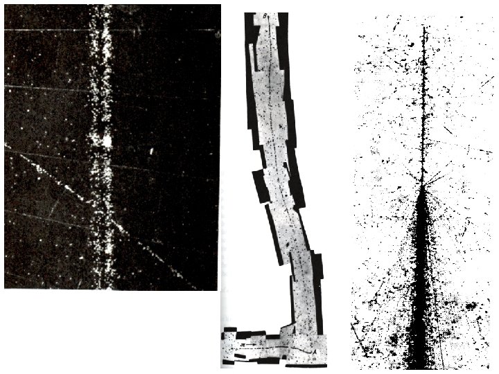
B-field points into page 1900 -01 Studying the deflection of these rays in magnetic fields, Becquerel and the Curies establish rays to be charged particles

1900 -01 Using the procedure developed by J. J. Thomson in 1887 Becquerel determined the ratio of charge q to mass m for : q/m = 1. 76× 1011 coulombs/kilogram identical to the electron! : q/m = 4. 8× 107 coulombs/kilogram 4000 times smaller!

Discharge Tube Thin-walled (0. 01 mm) glass tube Noting helium gas often found trapped in samples of radioactive minerals, Rutherford speculated that particles might be doubly ionized Helium atoms (He++) 1906 -1909 Rutherford and T. D. Royds develop their “alpha mousetrap” to collect alpha particles and show this yields a gas with the spectral emission lines of helium! to vacuum pump & Mercury supply Radium or Radon gas

Status of particle physics early 20 th century Electron J. J. Thomson 1898 nucleus ( proton) Ernest Rutherford 1908 -09 Henri Becquerel 1896 Ernest Rutherford 1899 P. Villard X-rays Wilhelm Roentgen 1895 1900

Periodic Table of the Elements Fe 26 55. 86 Co 27 58. 93 Ni 28 58. 71 Atomic mass values averaged over all isotopes in the proportion they naturally occur.

Through lead, ~1/4 of the elements come in “single species” Isotopes are chemically identical (not separable by any chemical means) but are physically different (mass) 6 The “last” 11 naturally occurring elements (Lead Uranium) Z=82 recur in 3 principal “radioactive series. ” 92

234 Th 90 234 Pa 91 234 U 92 230 Th 90 226 Ra 88 214 Pb 82 214 83 Bi 214 Po 84 82 Pb 210 Pb 82 210 83 Bi 210 Po 84 82 Pb 206 238 92 U “Uranium I” “Uranium II” “Radium B” “Radium G” 92 U 234 222 Rn 86 4. 5 109 years 2. 5 105 years 218 Po 84 U 238 U 234 radioactive Pb 214 stable Pb 206 82 Pb 214

Chemically separating the lead from various minerals (which suggested their origin) and comparing their masses: Thorite (thorium with traces if uranium and lead) 208 amu Pitchblende (containing uranium mineral and lead) 206 amu “ordinary” lead deposits are chiefly 207 amu

Masses are given in atomic mass units (amu) based on 6 C 12 = 12. 000000

Mass of bare hydrogen nucleus: 1. 00727 amu Mass of electron: 0. 000549 amu

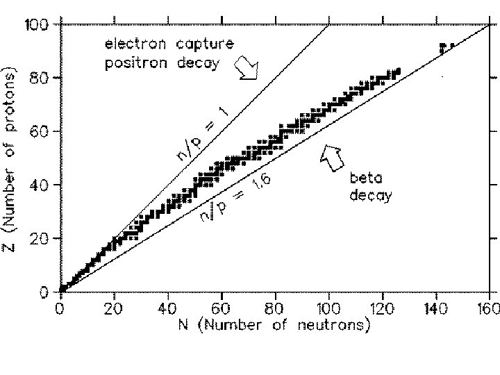
number of protons number of neutrons

Number surviving Radioactive atoms What does stand for?

log. N time Number surviving Radioactive atoms

for x measured in radians (not degrees!)

Let’s complete the table below (using a calculator) to check the “small angle approximation” (for angles not much bigger than ~15 -20 o) which ignores more than the 1 st term of the series Note: the x or (in radians) = ( /180 o) (in degrees) Angle (radians) 25 o 0 1 2 3 4 6 8 10 15 20 25 0 0. 017453293 0. 034906585 0. 052359878 0. 069813170 0. 104719755 0. 139626340 0. 174532952 0. 261799388 0. 349065850 0. 436332313 sin 0. 00000 0. 017452406 0. 034899497 0. 052335956 0. 069756473 0. 104528463 0. 139173101 0. 173648204 0. 258819045 0. 342020143 0. 422618262 97% accurate!

y=x y = x 3/6 y = x - x 3/6 + x 5/120 y = sin x y = x - x 3/6

Any power of e can be expanded as an infinite series Let’s compute some powers of e using just the above 5 terms of the series e 0 = 1 + 0 + 0 = 1 e 1 = 1 + 0. 500000 + 0. 166667 + 0. 041667 2. 708334 e 2 = 1 + 2. 000000 + 1. 333333 + 0. 666667 7. 000000 e 2 = 7. 3890560989…

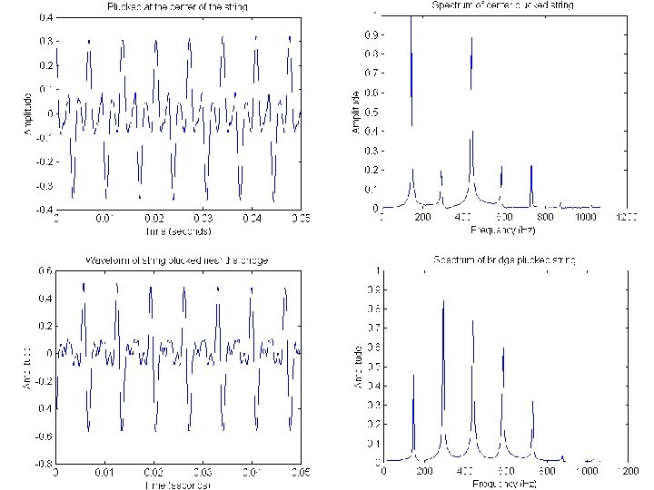
violin Piano, Concert C Clarinet, Concert C Miles Davis’ trumpet

A Fourier where series can be defined for any function over the interval 0 x 2 L Often easiest to treat n=0 cases separately

Compute the Fourier series of the SQUARE WAVE function f given by 2 Note: f(x) is an odd function ( i. e. f(-x) = -f(x) ) so f(x) cos nx will be as well, while f(x) sin nx will be even.

change of variables: x x' = x- periodicity: cos(X-n ) = (-1)ncos. X for n = 1, 3, 5, …

for n = 2, 4, 6, … for n = 1, 3, 5, … change of variables: x x' = nx

periodicity: cos(X-n ) = (-1)ncos. X for n = 1, 3, 5, …

for n = 2, 4, 6, … for n = 1, 3, 5, … change of variables: x x' = nx for odd n for n = 1, 3, 5, …

y 1 2 x

Leads you through a qualitative argument in building a square wave http: //mathforum. org/key/nucalc/fourier. html Add terms one by one (or as many as you want) to build fourier series approximation to a selection of periodic functions http: //www. jhu. edu/~signals/fourier 2/ Build Fourier series approximation to assorted periodic functions and listen to an audio playing the wave forms http: //www. falstad. com/fourier/ Customize your own sound synthesizer http: //www. phy. ntnu. edu. tw/java/sound. html

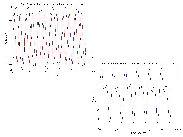
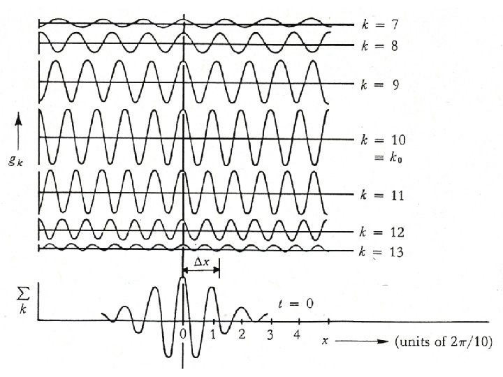
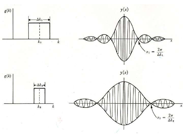
NOTE: The spatial distribution depends on the particular frequencies involved x 1 x k k = 2 Two waves of slightly different wavelength and frequency produce beats.

Fourier Transforms Generalization of ordinary “Fourier expansion” or “Fourier series” Note how this pairs canonically conjugate variables and t.

Fourier transforms do allow an explicit “closed” analytic form for the Dirac delta function

Let’s assume a wave packet tailored to be something like a Gaussian (or “Normal”) distribution Area within 1 1. 28 1. 64 1. 96 2 2. 58 3 4 68. 26% 80. 00% 95. 44% 99. 00% 99. 46% 99. 99% -2 -1 +1 +2

For well-behaved (continuous) functions (bounded at infiinity) 2/2 2 -x like f(x)=e Starting from: f(x) is bounded g'(x) oscillates in the complex plane over-all amplitude is damped at ± g(x)= i +kx e k

Similarly, starting from:

And so, specifically for a normal distribution: f(x)=e-x differentiating: from the relation just derived: Let’s Fourier transform THIS statement i. e. , apply: on both sides! 1 ~ ~ ~ -ikx F'(k)e dk 2 ~ 1 e-i(k-k)x dx 2 ~ (k – k) 2/2 2

~ 1 e-i(k-k)x dx 2 ~ (k – k) ~ selecting out k=k k rewriting as: 0 ' ' k ' dk' 0

Fourier transforms of one another Gaussian distribution about the origin Now, since: we expect: Both are of the form of a Gaussian! x k 1/

x k 1 or giving physical interpretation to the new variable x px h