The Evergreen Project The Promise of Polynomials to

The Evergreen Project: The Promise of Polynomials to Boost CSP/SAT Solvers* Karl J. Lieberherr Northeastern University Boston joint work with Ahmed Abdelmeged, Christine Hang and Daniel Rinehart UBC March 2007 Title inspired by a paper by Carla Gomes / David Shmoys 1

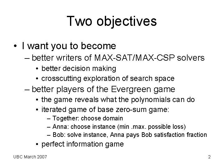
Two objectives • I want you to become – better writers of MAX-SAT/MAX-CSP solvers • better decision making • crosscutting exploration of search space – better players of the Evergreen game • the game reveals what the polynomials can do • iterated game of base zero-sum game: – Together: choose domain – Anna: choose instance (min. max. possible loss) – Bob: solve instance, Anna pays Bob satisfaction fraction • perfect information game UBC March 2007 2

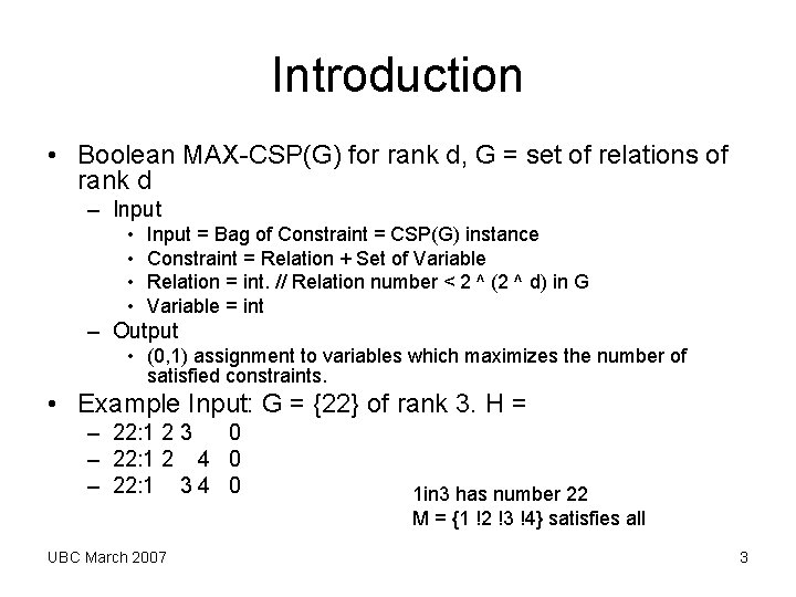
Introduction • Boolean MAX-CSP(G) for rank d, G = set of relations of rank d – Input • • Input = Bag of Constraint = CSP(G) instance Constraint = Relation + Set of Variable Relation = int. // Relation number < 2 ^ (2 ^ d) in G Variable = int – Output • (0, 1) assignment to variables which maximizes the number of satisfied constraints. • Example Input: G = {22} of rank 3. H = – 22: 1 2 3 0 – 22: 1 2 4 0 – 22: 1 3 4 0 UBC March 2007 1 in 3 has number 22 M = {1 !2 !3 !4} satisfies all 3

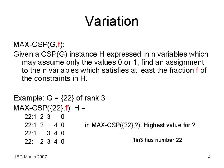
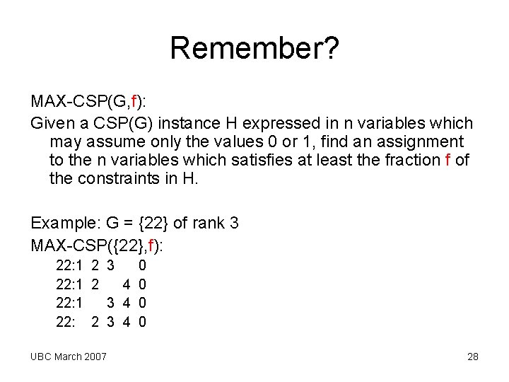
Variation MAX-CSP(G, f): Given a CSP(G) instance H expressed in n variables which may assume only the values 0 or 1, find an assignment to the n variables which satisfies at least the fraction f of the constraints in H. Example: G = {22} of rank 3 MAX-CSP({22}, f): H = 22: 1 2 3 0 22: 1 2 4 0 in MAX-CSP({22}, ? ). Highest value for ? 22: 1 3 4 0 1 in 3 has number 22 22: 2 3 4 0 UBC March 2007 4

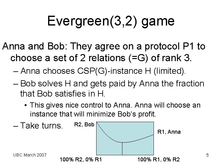
Evergreen(3, 2) game Anna and Bob: They agree on a protocol P 1 to choose a set of 2 relations (=G) of rank 3. – Anna chooses CSP(G)-instance H (limited). – Bob solves H and gets paid by Anna the fraction that Bob satisfies in H. • This gives nice control to Anna will choose an instance that will minimize Bob’s profit. – Take turns. UBC March 2007 R 2, Bob 100% R 2, 0% R 1, Anna 100% R 1, 0% R 2 5

Protocol choice • Randomly choose R 1 and R 2 (independently) between 1 and 255 (Throw two dice choosing relations). UBC March 2007 6

Tell me • How would you react as Anna? – The relations 22 and 22 have been chosen. – You must create a CSP({22}) instance with 1000 variables in which only the smallest possible fraction can be satisfied. – What kind of instance will this be? • What kind of algorithm should Bob use to maximize its payoff? • Should any MAX-CSP solver be able to maximize Bob’s profit? How well does MAX-SAT (e. g. , yices, UBC March 2007 ubcsat) or MAX-CSP solvers do on symmetric 7 instances ? ? ?

Game strategy in a nutshell • Choose G={R 1, R 2} randomly. • Anna chooses instance so that payoff is minimized. • Bob finds solution so that payoff is maximized (Solve MAX-CSP(G)) • Take turns: Choose G= … Bob chooses … • Requires thorough understanding of MAXCSP(G) problem domain. Requires an excellent MAX-CSP(G) solver. UBC March 2007 8

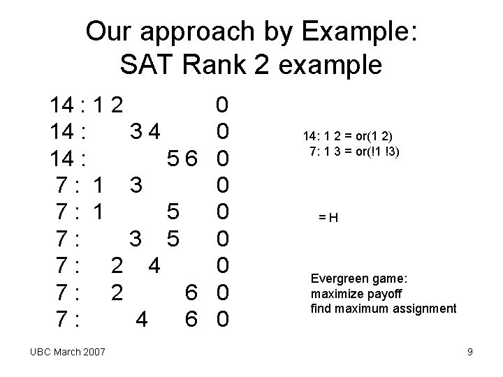
Our approach by Example: SAT Rank 2 example 14 : 1 2 0 14 : 3 4 0 14 : 5 6 0 7 : 1 3 0 7 : 1 5 0 7 : 3 5 0 7 : 2 4 0 7 : 2 6 0 7 : 4 6 0 UBC March 2007 14: 1 2 = or(1 2) 7: 1 3 = or(!1 !3) = H Evergreen game: maximize payoff find maximum assignment 9

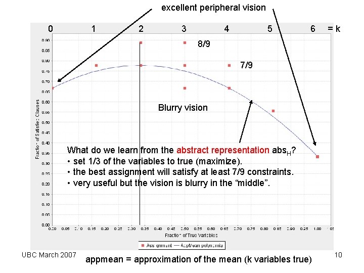
excellent peripheral vision 0 1 2 3 4 5 6 = k 8/9 7/9 Blurry vision What do we learn from the abstract representation abs. H? • set 1/3 of the variables to true (maximize). • the best assignment will satisfy at least 7/9 constraints. • very useful but the vision is blurry in the “middle”. UBC March 2007 appmean = approximation of the mean (k variables true) 10

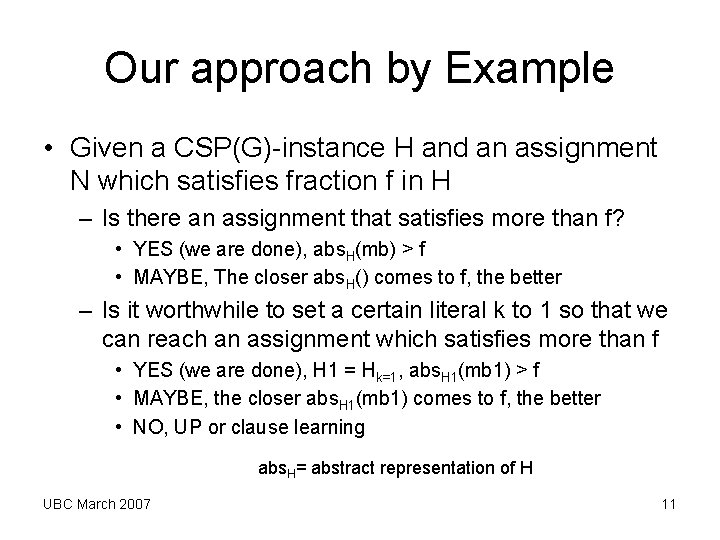
Our approach by Example • Given a CSP(G)-instance H and an assignment N which satisfies fraction f in H – Is there an assignment that satisfies more than f? • YES (we are done), abs. H(mb) > f • MAYBE, The closer abs. H() comes to f, the better – Is it worthwhile to set a certain literal k to 1 so that we can reach an assignment which satisfies more than f • YES (we are done), H 1 = Hk=1, abs. H 1(mb 1) > f • MAYBE, the closer abs. H 1(mb 1) comes to f, the better • NO, UP or clause learning abs. H= abstract representation of H UBC March 2007 11

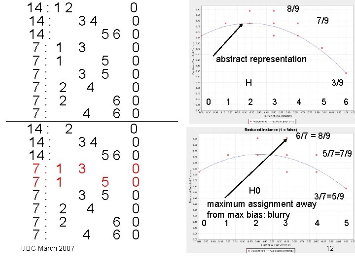
14 : 1 2 0 14 : 3 4 0 14 : 5 6 0 7 : 1 3 0 7 : 1 5 0 7 : 3 5 0 7 : 2 4 0 7 : 2 6 0 7 : 4 6 0 14 : 2 0 14 : 3 4 0 14 : 5 6 0 7 : 1 3 0 7 : 1 5 0 7 : 3 5 0 7 : 2 4 0 7 : 2 6 0 7 : 4 6 0 UBC March 2007 8/9 7/9 abstract representation H 3/9 0 1 2 3 4 5 6 6/7 = 8/9 5/7=7/9 H 0 3/7=5/9 maximum assignment away from max bias: blurry 0 1 2 3 4 5 12

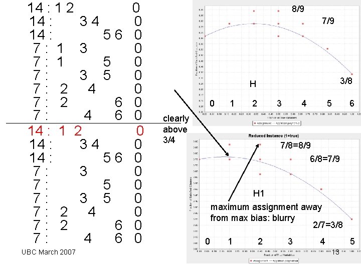
14 : 1 2 0 14 : 3 4 0 14 : 5 6 0 7 : 1 3 0 7 : 1 5 0 7 : 3 5 0 7 : 2 4 0 7 : 2 6 0 7 : 4 6 0 14 : 1 2 0 14 : 3 4 0 14 : 5 6 0 7 : 3 0 7 : 5 0 7 : 3 5 0 7 : 2 4 0 7 : 2 6 0 7 : 4 6 0 UBC March 2007 8/9 7/9 3/8 H 0 1 2 3 4 5 6 clearly above 3/4 7/8=8/9 6/8=7/9 H 1 maximum assignment away from max bias: blurry 2/7=3/8 0 1 2 3 4 5 13

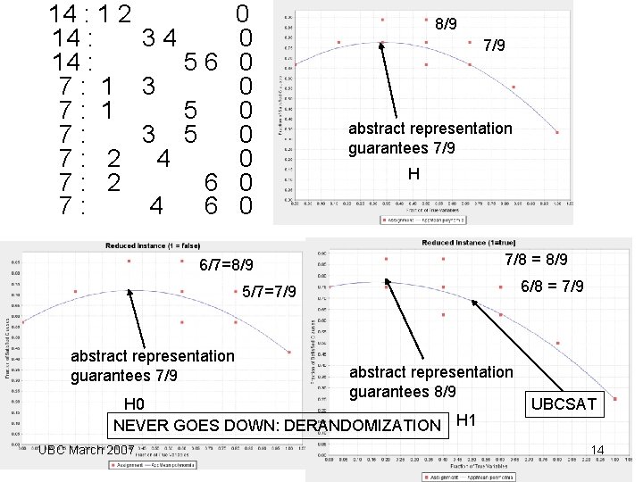
14 : 1 2 0 14 : 3 4 0 14 : 5 6 0 7 : 1 3 0 7 : 1 5 0 7 : 3 5 0 7 : 2 4 0 7 : 2 6 0 7 : 4 6 0 8/9 7/9 abstract representation guarantees 7/9 H 7/8 = 8/9 6/7=8/9 6/8 = 7/9 5/7=7/9 abstract representation guarantees 8/9 H 0 NEVER GOES DOWN: DERANDOMIZATION H 1 UBC March 2007 UBCSAT 14

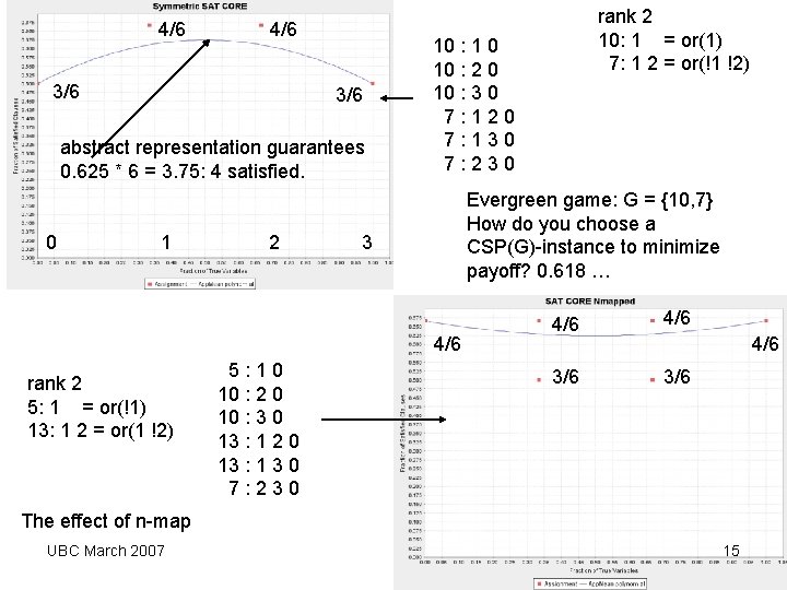
4/6 3/6 abstract representation guarantees 0. 625 * 6 = 3. 75: 4 satisfied. 10 : 1 0 10 : 2 0 10 : 3 0 7 : 1 2 0 7 : 1 3 0 7 : 2 3 0 Evergreen game: G = {10, 7} How do you choose a CSP(G)-instance to minimize payoff? 0. 618 … 0 1 2 3 4/6 rank 2 5: 1 = or(!1) 13: 1 2 = or(1 !2) 5 : 1 0 10 : 2 0 10 : 3 0 13 : 1 2 0 13 : 1 3 0 7 : 2 3 0 rank 2 10: 1 = or(1) 7: 1 2 = or(!1 !2) 4/6 3/6 4/6 The effect of n-map UBC March 2007 15

First Impression • The abstract representation = look-ahead polynomials seems useful for guiding the search. • The look-ahead polynomials give us averages: the guidance can be misleading because of outliers. • But how can we compute the look-ahead polynomials? How do the polynomials help play the Evergreen(3, 2) game? UBC March 2007 16

Where we are • • Introduction Look-forward Look-backward SPOT: how to use the look-ahead polynomials together with superresolution. UBC March 2007 17

Look Forward • Why? – To make informed decisions – To play the Evergreen game • How? – Abstract representation based on look-ahead polynomials UBC March 2007 18

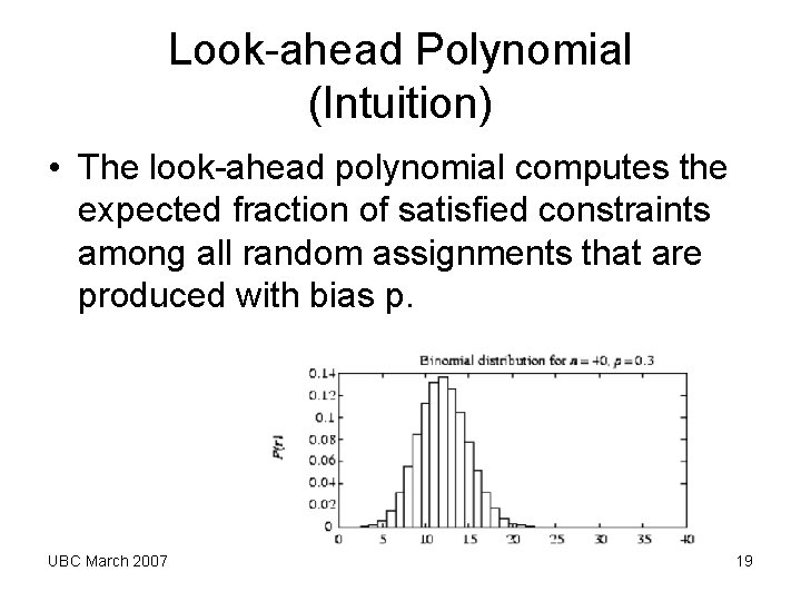
Look-ahead Polynomial (Intuition) • The look-ahead polynomial computes the expected fraction of satisfied constraints among all random assignments that are produced with bias p. UBC March 2007 19

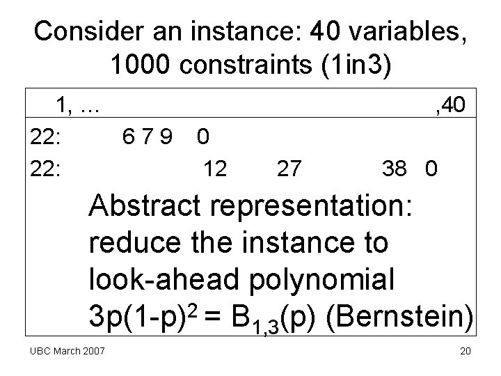
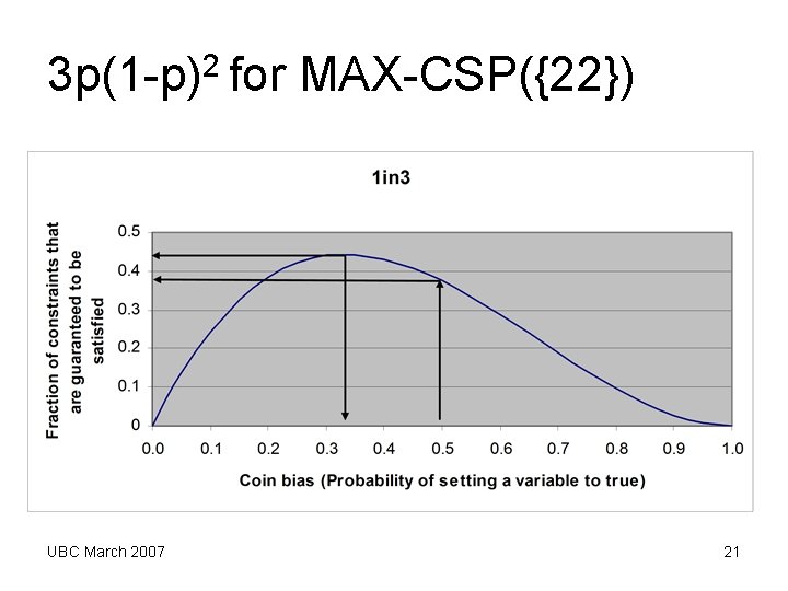
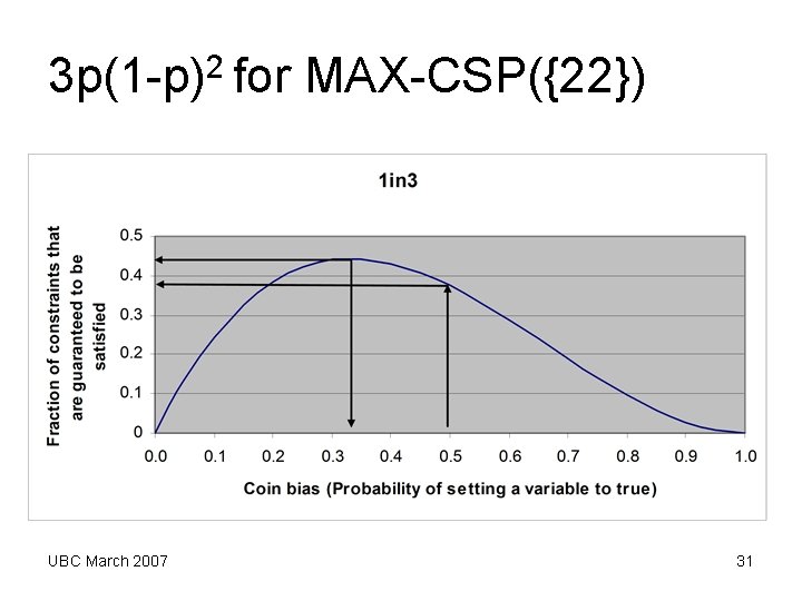
Consider an instance: 40 variables, 1000 constraints (1 in 3) 1, … , 40 22: 6 7 9 0 22: 12 27 38 0 Abstract representation: reduce the instance to look-ahead polynomial 2 3 p(1 -p) = B 1, 3(p) (Bernstein) UBC March 2007 20

3 p(1 -p)2 for MAX-CSP({22}) UBC March 2007 21

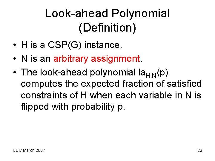
Look-ahead Polynomial (Definition) • H is a CSP(G) instance. • N is an arbitrary assignment. • The look-ahead polynomial la. H, N(p) computes the expected fraction of satisfied constraints of H when each variable in N is flipped with probability p. UBC March 2007 22

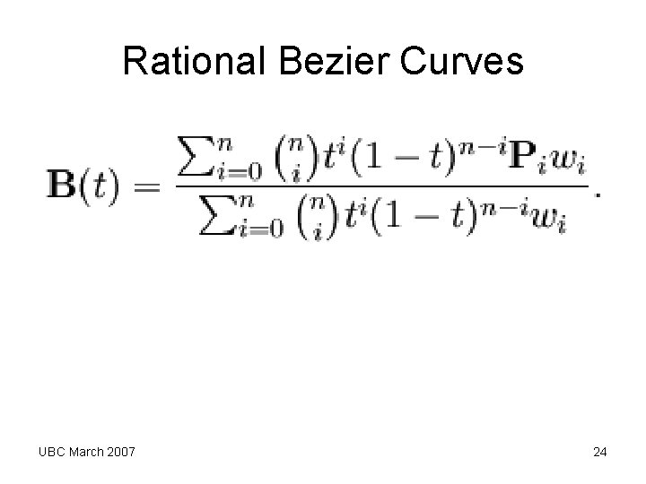
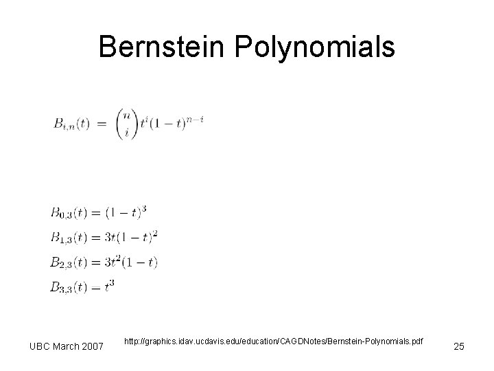
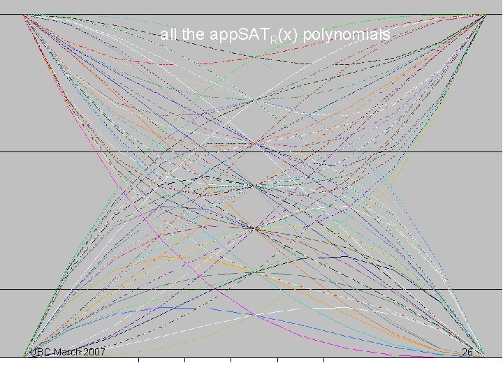
The general case MAX-CSP(G) G = {R 1, … }, t. R(F) = fraction of constraints in F that use R. x = p UBC March 2007 app. SATR(x) over all R is a super set of the Bernstein polynomials (computer graphics, weighted sum of Bernstein polynomials) 23

Rational Bezier Curves UBC March 2007 24

Bernstein Polynomials UBC March 2007 http: //graphics. idav. ucdavis. edu/education/CAGDNotes/Bernstein-Polynomials. pdf 25

all the app. SATR(x) polynomials UBC March 2007 26

Look-ahead Polynomial in Action • Focus on purely mathematical question first • Algorithmic solution will follow • Mathematical question: Given a CSP(G) instance. For which fractions f is there always an assignment satisfying fraction f of the constraints? In which constraint systems is it impossible to satisfy many constraints? UBC March 2007 27

Remember? MAX-CSP(G, f): Given a CSP(G) instance H expressed in n variables which may assume only the values 0 or 1, find an assignment to the n variables which satisfies at least the fraction f of the constraints in H. Example: G = {22} of rank 3 MAX-CSP({22}, f): 22: 1 2 3 0 22: 1 2 4 0 22: 1 3 4 0 22: 2 3 4 0 UBC March 2007 28

Mathematical Critical Transition Point MAX-CSP({22}, f): For f ≤ u: problem has always a solution For f ≥ u + e: problem has not always a solution, e>0. 1 not always (solid) u = critical transition point always (fluid) 0 UBC March 2007 29

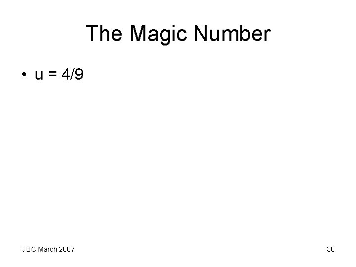
The Magic Number • u = 4/9 UBC March 2007 30

3 p(1 -p)2 for MAX-CSP({22}) UBC March 2007 31

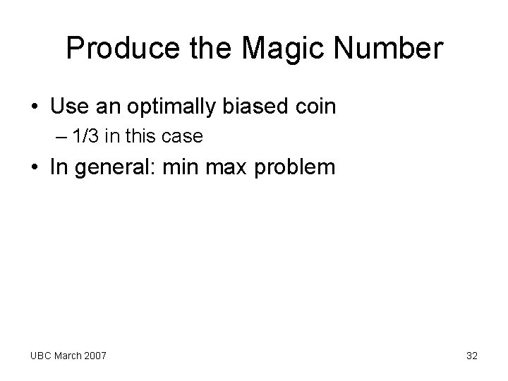
Produce the Magic Number • Use an optimally biased coin – 1/3 in this case • In general: min max problem UBC March 2007 32

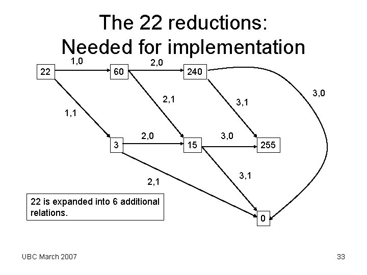
The 22 reductions: Needed for implementation 1, 0 22 60 2, 0 240 2, 1 3, 0 3, 1 1, 1 3 2, 0 2, 1 22 is expanded into 6 additional relations. UBC March 2007 15 3, 0 255 3, 1 0 33

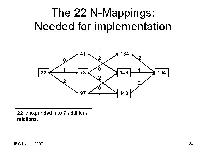
The 22 N-Mappings: Needed for implementation 41 0 22 1 73 2 97 1 2 0 1 134 146 2 1 104 0 148 22 is expanded into 7 additional relations. UBC March 2007 34

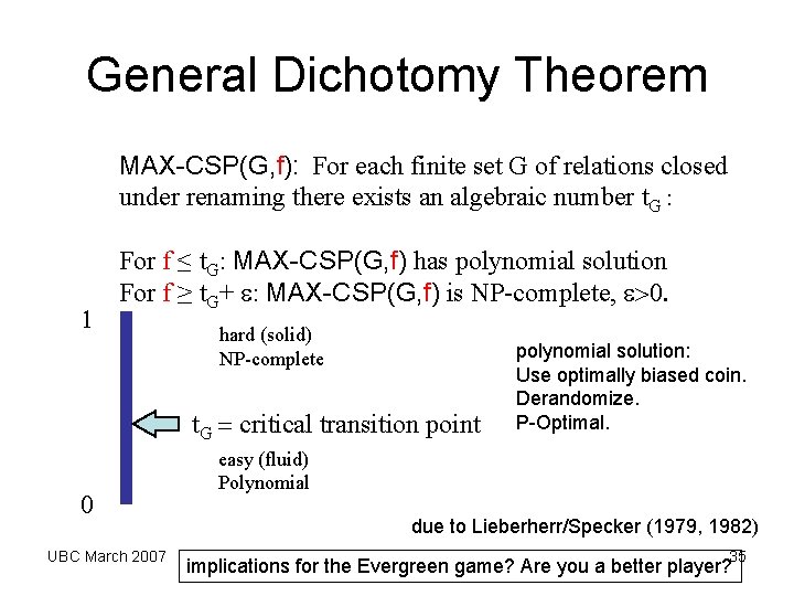
General Dichotomy Theorem MAX-CSP(G, f): For each finite set G of relations closed under renaming there exists an algebraic number t. G : 1 For f ≤ t. G: MAX-CSP(G, f) has polynomial solution For f ≥ t. G+ e: MAX-CSP(G, f) is NP-complete, e>0. hard (solid) NP-complete t. G = critical transition point 0 UBC March 2007 polynomial solution: Use optimally biased coin. Derandomize. P-Optimal. easy (fluid) Polynomial due to Lieberherr/Specker (1979, 1982) 35 implications for the Evergreen game? Are you a better player?

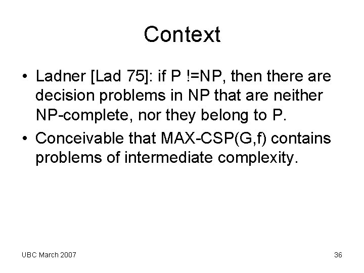
Context • Ladner [Lad 75]: if P !=NP, then there are decision problems in NP that are neither NP-complete, nor they belong to P. • Conceivable that MAX-CSP(G, f) contains problems of intermediate complexity. UBC March 2007 36

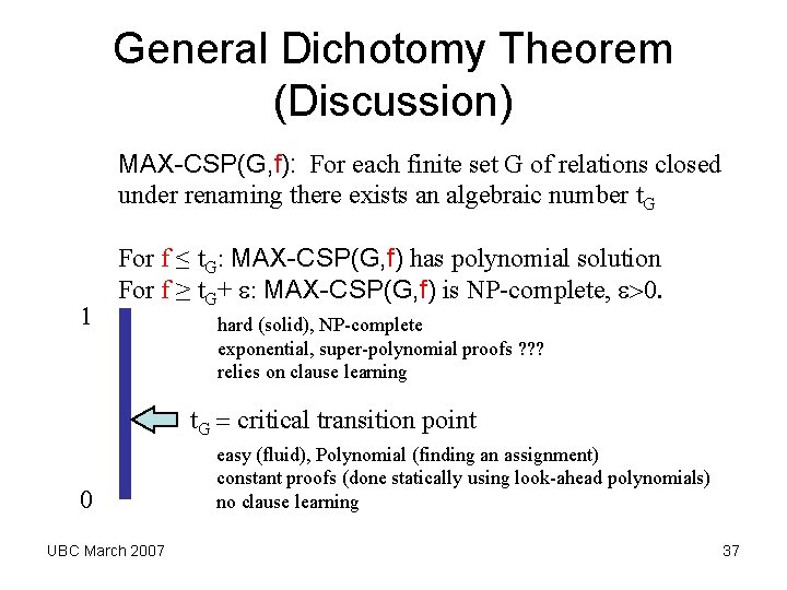
General Dichotomy Theorem (Discussion) MAX-CSP(G, f): For each finite set G of relations closed under renaming there exists an algebraic number t. G 1 For f ≤ t. G: MAX-CSP(G, f) has polynomial solution For f ≥ t. G+ e: MAX-CSP(G, f) is NP-complete, e>0. hard (solid), NP-complete exponential, super-polynomial proofs ? ? ? relies on clause learning t. G = critical transition point 0 UBC March 2007 easy (fluid), Polynomial (finding an assignment) constant proofs (done statically using look-ahead polynomials) no clause learning 37

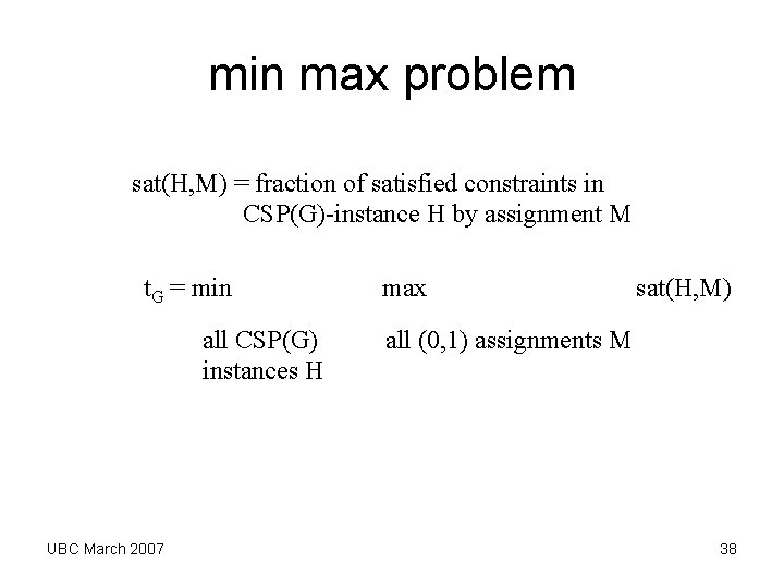
min max problem sat(H, M) = fraction of satisfied constraints in CSP(G)-instance H by assignment M t. G = min all CSP(G) instances H UBC March 2007 max sat(H, M) all (0, 1) assignments M 38

Problem reductions are the key • Solution to simpler problem implies solution to original problem. UBC March 2007 39

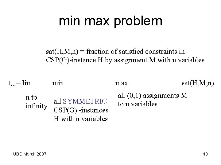
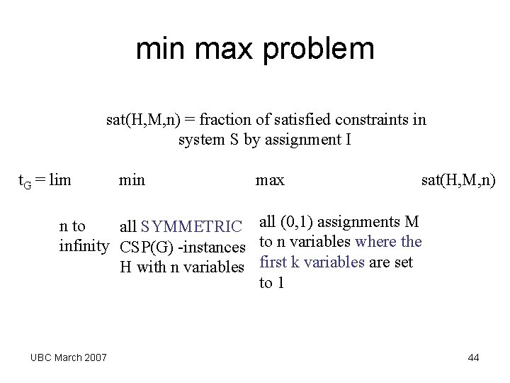
min max problem sat(H, M, n) = fraction of satisfied constraints in CSP(G)-instance H by assignment M with n variables. t. G = lim min n to all SYMMETRIC infinity CSP(G) -instances H with n variables UBC March 2007 max sat(H, M, n) all (0, 1) assignments M to n variables 40

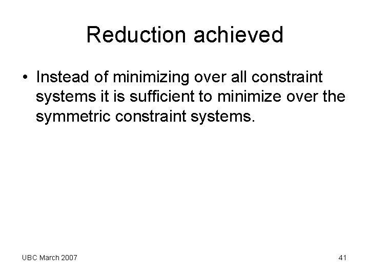
Reduction achieved • Instead of minimizing over all constraint systems it is sufficient to minimize over the symmetric constraint systems. UBC March 2007 41

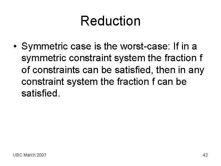
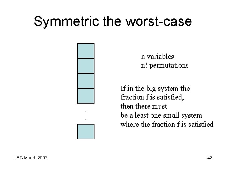
Reduction • Symmetric case is the worst-case: If in a symmetric constraint system the fraction f of constraints can be satisfied, then in any constraint system the fraction f can be satisfied. UBC March 2007 42

Symmetric the worst-case n variables n! permutations . . UBC March 2007 If in the big system the fraction f is satisfied, then there must be a least one small system where the fraction f is satisfied 43

min max problem sat(H, M, n) = fraction of satisfied constraints in system S by assignment I t. G = lim min max sat(H, M, n) n to all SYMMETRIC all (0, 1) assignments M infinity CSP(G) -instances to n variables where the H with n variables first k variables are set to 1 UBC March 2007 44

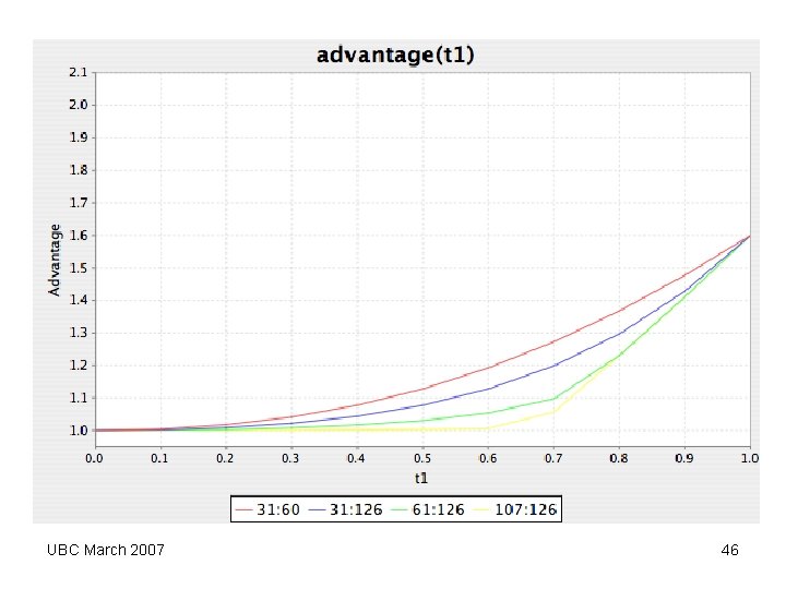
Observations • The look-ahead polynomial look-forward approach has not been used in state-ofthe-art MAX-SAT and Boolean MAX-CSP solvers. • Often a fair coin is used. The optimally biased coin is often significantly better. UBC March 2007 45

UBC March 2007 46

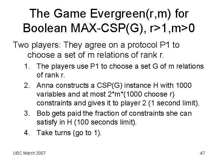
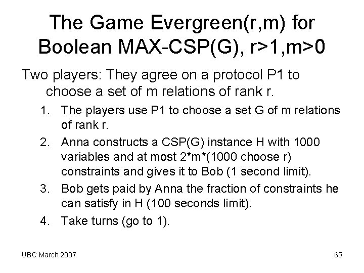
The Game Evergreen(r, m) for Boolean MAX-CSP(G), r>1, m>0 Two players: They agree on a protocol P 1 to choose a set of m relations of rank r. 1. The players use P 1 to choose a set G of m relations of rank r. 2. Anna constructs a CSP(G) instance H with 1000 variables and at most 2*m*(1000 choose r) constraints and gives it to player 2 (1 second limit). 3. Bob gets paid the fraction of constraints she can satisfy in H (100 seconds limit). 4. Take turns (go to 1). UBC March 2007 47

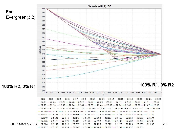
For Evergreen(3, 2) 100% R 2, 0% R 1 UBC March 2007 100% R 1, 0% R 2 48

Evergreen(3, 2) protocol possibilities • Variant 1 – Player Bob chooses both relations G – Player Anna chooses CSP(G) instance H. – Player Bob solves H and gets paid by Anna. • This gives too much control to Bob can choose two odd relations which guarantees him a pay of 1 independent of how Anna chooses the instance H. UBC March 2007 49

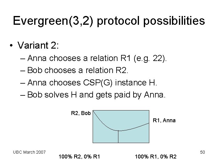
Evergreen(3, 2) protocol possibilities • Variant 2: – Anna chooses a relation R 1 (e. g. 22). – Bob chooses a relation R 2. – Anna chooses CSP(G) instance H. – Bob solves H and gets paid by Anna. R 2, Bob R 1, Anna UBC March 2007 100% R 2, 0% R 1 100% R 1, 0% R 2 50

Problem with variant 2 • Anna can just ignore relation R 2. • Gives Anna too much control because the payoff for Bob depends only on R 1 chosen by Anna (and the quality of the solver that Bob uses). UBC March 2007 51

Protocol choice: variant 3 • Randomly choose R 1 and R 2 (independently) between 1 and 255 (Throw two dice). UBC March 2007 52

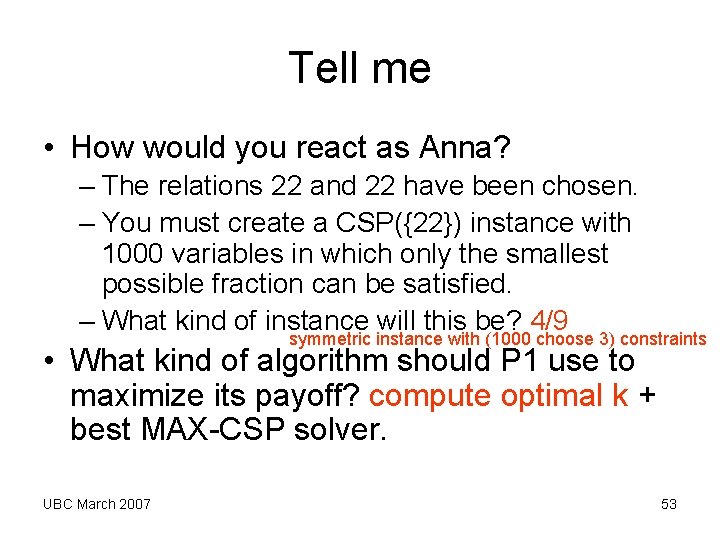
Tell me • How would you react as Anna? – The relations 22 and 22 have been chosen. – You must create a CSP({22}) instance with 1000 variables in which only the smallest possible fraction can be satisfied. – What kind of instance will this be? 4/9 symmetric instance with (1000 choose 3) constraints • What kind of algorithm should P 1 use to maximize its payoff? compute optimal k + best MAX-CSP solver. UBC March 2007 53

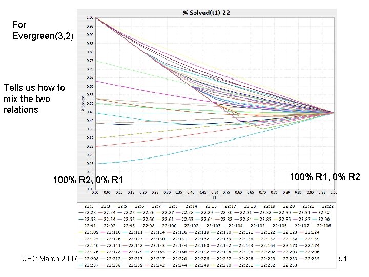
For Evergreen(3, 2) Tells us how to mix the two relations 100% R 2, 0% R 1 UBC March 2007 100% R 1, 0% R 2 54

Role of t. G in the Evergreen(3, 2) game • 1: Instance construction: Choose a CSP(G) instance so that only the fraction t. G can be satisfied: symmetric formula. • 2: Choose an algorithm so that at least the fraction t. G is satisfied. (2 gets paid t. G from 1). UBC March 2007 55

Game strategy in a nutshell • Anna: Best: Choose t. G instance • Bob: Get’s paid t. G • etc. UBC March 2007 56

Additional Information • Rich literature on clause learning in SAT and CSP solver domain. Superresolution is the most general form of clause learning with restarts. • Papers on look-ahead polynomials and superresolution: http: //www. ccs. neu. edu/research/demeter/ papers/publications. html UBC March 2007 57

Additional Information • Useful unpublished paper on look-ahead polynomials: http: //www. ccs. neu. edu/research/demeter/ biblio/partial-sat-II. html • Technical report on the topic of this talk: http: //www. ccs. neu. edu/research/demeter/ biblio/POpt. MAXCSP. html UBC March 2007 58

Future work • Exploring best combination of look-forward and look-back techniques. • Find all maximum-assignments or estimate their number. • Robustness of maximum assignments. • Are our MAX-CSP solvers useful for reasoning about biological pathways? UBC March 2007 59

Conclusions • Presented SPOT, a family of MAX-CSP solvers based on look-ahead polynomials and non-chronological backtracking. • SPOT has a desirable property: P-optimal. • SPOT can be implemented very efficiently. • Preliminary experimental results are encouraging. A lot more work is needed to assess the practical value of the lookahead polynomials. UBC March 2007 60

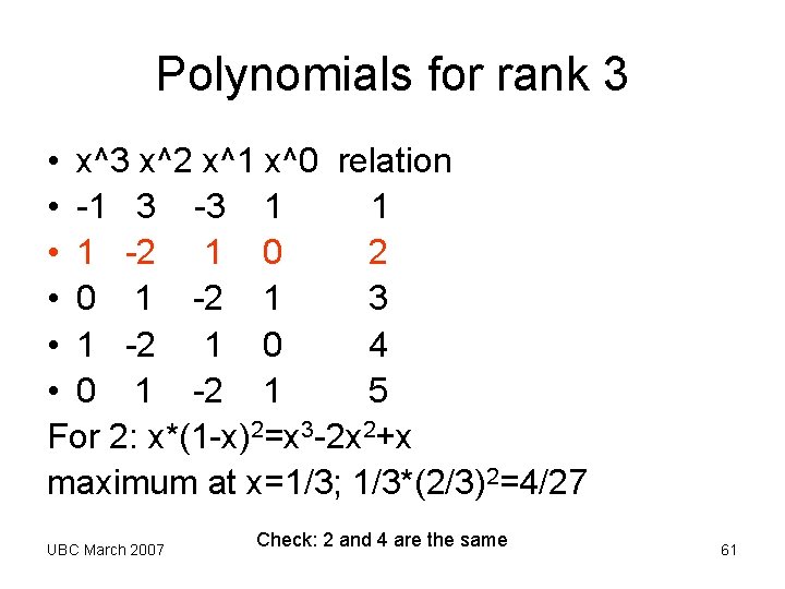
Polynomials for rank 3 • x^3 x^2 x^1 x^0 relation • -1 3 -3 1 • 1 -2 1 0 2 • 0 1 -2 1 3 • 1 -2 1 0 4 • 0 1 -2 1 5 For 2: x*(1 -x)2=x 3 -2 x 2+x maximum at x=1/3; 1/3*(2/3)2=4/27 UBC March 2007 Check: 2 and 4 are the same 61

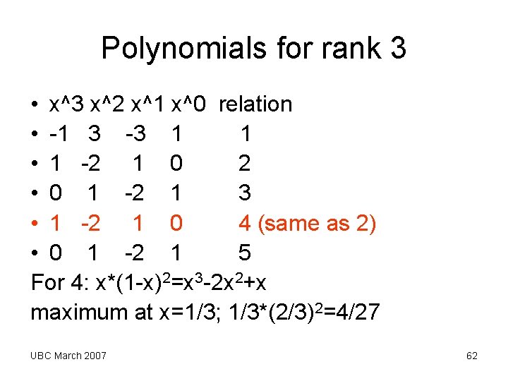
Polynomials for rank 3 • x^3 x^2 x^1 x^0 relation • -1 3 -3 1 • 1 -2 1 0 2 • 0 1 -2 1 3 • 1 -2 1 0 4 (same as 2) • 0 1 -2 1 5 For 4: x*(1 -x)2=x 3 -2 x 2+x maximum at x=1/3; 1/3*(2/3)2=4/27 UBC March 2007 62

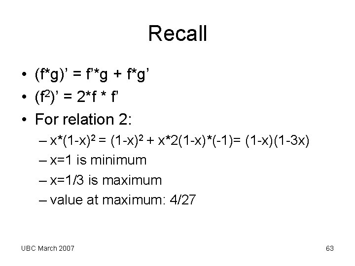
Recall • (f*g)’ = f’*g + f*g’ • (f 2)’ = 2*f * f’ • For relation 2: – x*(1 -x)2 = (1 -x)2 + x*2(1 -x)*(-1)= (1 -x)(1 -3 x) – x=1 is minimum – x=1/3 is maximum – value at maximum: 4/27 UBC March 2007 63

Harold • • • concern: intension, extension: query, predicate extension = intension(software) Harold Ossher: confirmed pointcuts UBC March 2007 64

The Game Evergreen(r, m) for Boolean MAX-CSP(G), r>1, m>0 Two players: They agree on a protocol P 1 to choose a set of m relations of rank r. 1. The players use P 1 to choose a set G of m relations of rank r. 2. Anna constructs a CSP(G) instance H with 1000 variables and at most 2*m*(1000 choose r) constraints and gives it to Bob (1 second limit). 3. Bob gets paid by Anna the fraction of constraints he can satisfy in H (100 seconds limit). 4. Take turns (go to 1). UBC March 2007 65

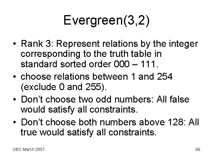
Evergreen(3, 2) • Rank 3: Represent relations by the integer corresponding to the truth table in standard sorted order 000 – 111. • choose relations between 1 and 254 (exclude 0 and 255). • Don’t choose two odd numbers: All false would satisfy all constraints. • Don’t choose both numbers above 128: All true would satisfy all constraints. UBC March 2007 66

How to play Evergreen(3, 2) • G = {R 1, R 2} is given (by some protocol) • Anna: compute t=(t 1, t 2) so that max appmeant(x) for x in [0, 1] is minimum. Construct a symmetric instance SYMG(t) H. • Bob: Solves H. UBC March 2007 67

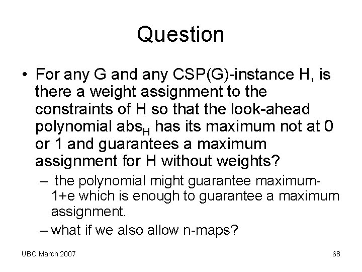
Question • For any G and any CSP(G)-instance H, is there a weight assignment to the constraints of H so that the look-ahead polynomial abs. H has its maximum not at 0 or 1 and guarantees a maximum assignment for H without weights? – the polynomial might guarantee maximum 1+e which is enough to guarantee a maximum assignment. – what if we also allow n-maps? UBC March 2007 68

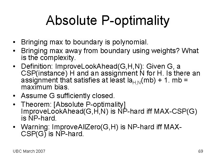
Absolute P-optimality • Bringing max to boundary is polynomial. • Bringing max away from boundary using weights? What is the complexity. • Definition: Improve. Look. Ahead(G, H, N): Given G, a CSP(instance) H and an assignment N for H. Is there an assignment that satisfies at least la. H, N(mb) + 1. mb = maximum bias. • Assume G sufficiently closed. • Theorem: [Absolute P-optimality] Improve. Look. Ahead(G, H, N) is NP-hard iff MAX-CSP(G) is NP-hard. • Warning: Improve. All. Zero(G, H) is NP-hard iff MAXCSP(G) is NP-hard. UBC March 2007 69

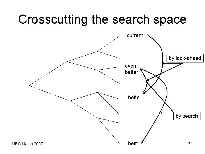
Exploring the search space • Look-ahead polynomials don’t eliminate parts of the search space. • They crosscut the search space early in the search process. Whenever the lookahead polynomial guarantees more than the currently best assignment, we can cut across the search space but might have to get back to the part we jumped over. UBC March 2007 70

Crosscutting the search space current by look-ahead even better by search UBC March 2007 best 71

Early better than later • Look-ahead polynomials are more useful early in the search. • Later in the search the maximum will be at 0 or 1. • Look-ahead polynomials will make mistakes which are compensated by superresolvents. • Superresolvents cut part of the search space and they help the look-ahead polynomials to eliminate the mistakes. UBC March 2007 72

Requirements for algorithms and properties to work • Relative P-optimality • Absolute P-optimality – G needs to be closed under renaming and reductions and n-maps • Look-ahead polynomials – improve assignments: closed under n-maps and reductions UBC March 2007 73

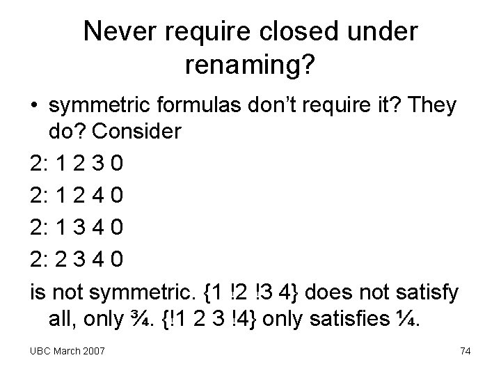
Never require closed under renaming? • symmetric formulas don’t require it? They do? Consider 2: 1 2 3 0 2: 1 2 4 0 2: 1 3 4 0 2: 2 3 4 0 is not symmetric. {1 !2 !3 4} does not satisfy all, only ¾. {!1 2 3 !4} only satisfies ¼. UBC March 2007 74

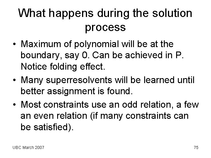
What happens during the solution process • Maximum of polynomial will be at the boundary, say 0. Can be achieved in P. Notice folding effect. • Many superresolvents will be learned until better assignment is found. • Most constraints use an odd relation, a few an even relation (if many constraints can be satisfied). UBC March 2007 75

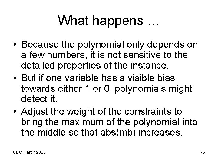
What happens … • Because the polynomial only depends on a few numbers, it is not sensitive to the detailed properties of the instance. • But if one variable has a visible bias towards either 1 or 0, polynomials might detect it. • Adjust the weight of the constraints to bring the maximum of the polynomial into the middle so that abs(mb) increases. UBC March 2007 76

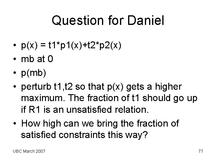
Question for Daniel • • p(x) = t 1*p 1(x)+t 2*p 2(x) mb at 0 p(mb) perturb t 1, t 2 so that p(x) gets a higher maximum. The fraction of t 1 should go up if R 1 is an unsatisfied relation. • How high can we bring the fraction of satisfied constraints this way? UBC March 2007 77

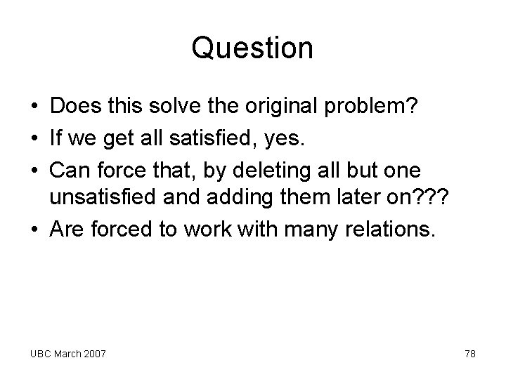
Question • Does this solve the original problem? • If we get all satisfied, yes. • Can force that, by deleting all but one unsatisfied and adding them later on? ? ? • Are forced to work with many relations. UBC March 2007 78

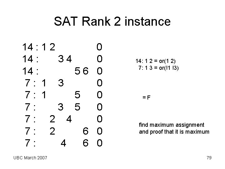
SAT Rank 2 instance 14 : 1 2 0 14 : 3 4 0 14 : 5 6 0 7 : 1 3 0 7 : 1 5 0 7 : 3 5 0 7 : 2 4 0 7 : 2 6 0 7 : 4 6 0 UBC March 2007 14: 1 2 = or(1 2) 7: 1 3 = or(!1 !3) = F find maximum assignment and proof that it is maximum 79

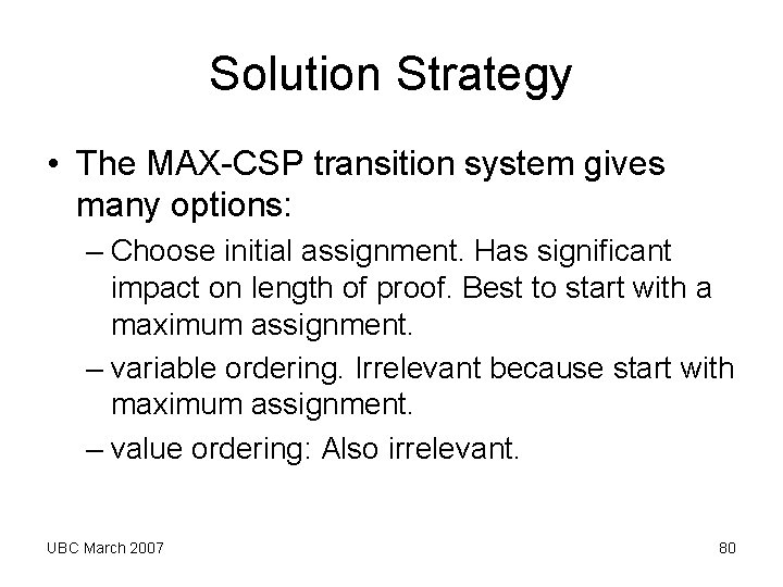
Solution Strategy • The MAX-CSP transition system gives many options: – Choose initial assignment. Has significant impact on length of proof. Best to start with a maximum assignment. – variable ordering. Irrelevant because start with maximum assignment. – value ordering: Also irrelevant. UBC March 2007 80

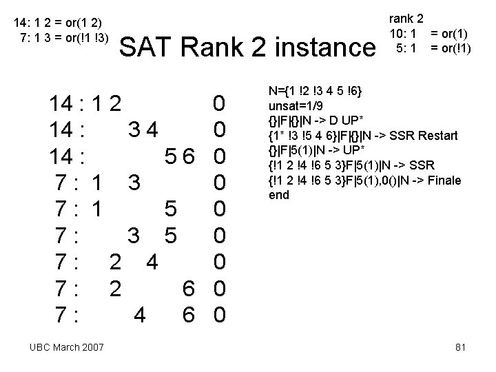
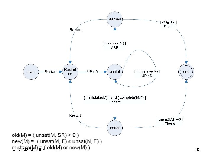
14: 1 2 = or(1 2) 7: 1 3 = or(!1 !3) SAT Rank 2 instance 14 : 1 2 0 14 : 3 4 0 14 : 5 6 0 7 : 1 3 0 7 : 1 5 0 7 : 3 5 0 7 : 2 4 0 7 : 2 6 0 7 : 4 6 0 UBC March 2007 rank 2 10: 1 = or(1) 5: 1 = or(!1) N={1 !2 !3 4 5 !6} unsat=1/9 {}|F|{}|N -> D UP* {1* !3 !5 4 6}|F|{}|N -> SSR Restart {}|F|5(1)|N -> UP* {!1 2 !4 !6 5 3}F|5(1)|N -> SSR {!1 2 !4 !6 5 3}F|5(1), 0()|N -> Finale end 81

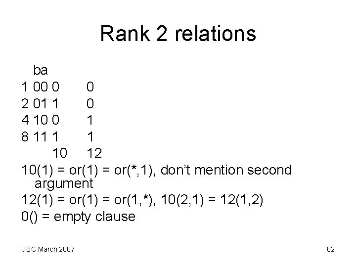
Rank 2 relations ba 1 00 0 0 2 01 1 0 4 10 0 1 8 11 1 1 10 12 10(1) = or(*, 1), don’t mention second argument 12(1) = or(1, *), 10(2, 1) = 12(1, 2) 0() = empty clause UBC March 2007 82

UBC March 2007 83

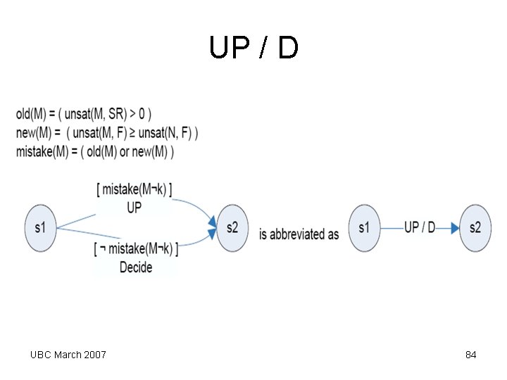
UP / D UBC March 2007 84

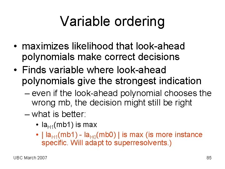
Variable ordering • maximizes likelihood that look-ahead polynomials make correct decisions • Finds variable where look-ahead polynomials give the strongest indication – even if the look-ahead polynomial chooses the wrong mb, the decision might still be right – what is better: • la. H 1(mb 1) is max • | la. H 1(mb 1) - la. H 0(mb 0) | is max (is more instance specific. Will adapt to superresolvents. ) UBC March 2007 85

mean versus appmean • mean does less averaging, so it is preferred? • appmean looks at the neighborhood of x*n UBC March 2007 86

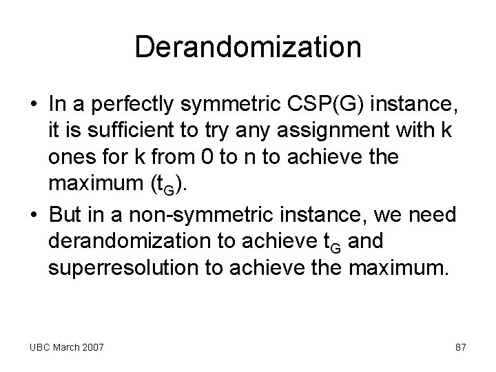
Derandomization • In a perfectly symmetric CSP(G) instance, it is sufficient to try any assignment with k ones for k from 0 to n to achieve the maximum (t. G). • But in a non-symmetric instance, we need derandomization to achieve t. G and superresolution to achieve the maximum. UBC March 2007 87

The Game Evergreen. TM(r, m) for Boolean MAX-CSP(G), r>1, m>0 Two players: They agree on a protocol P 1 to choose a set of m relations of rank r. 1. 2. 3. 4. The players use P 1 to choose a set G of m relations of rank r. Anna constructs a CSP(G) instance H with 1000 variables and at most 2*m*(1000 choose r) constraints and gives it to Bob (1 second limit). Anna knows the maximum assignment and has a proof for maximality but keeps it secret until Bob gives response. Bob gets paid the fraction of constraints he can satisfy in H relative to the maximum number that can be satisfied (100 seconds limit). Take turns (go to 1). UBC March 2007 TM = true maximum 88

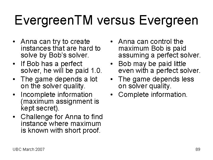
Evergreen. TM versus Evergreen • Anna can try to create instances that are hard to solve by Bob’s solver. • If Bob has a perfect solver, he will be paid 1. 0. • The game depends a lot on the solver quality. • Incomplete information (maximum assignment is kept secret). • Challenge for Anna to find instance where maximum is known with short proof. UBC March 2007 • Anna can control the maximum Bob is paid assuming a perfect solver. • Bob may be paid little even with a perfect solver. • The game depends less on solver quality. • Complete information. 89

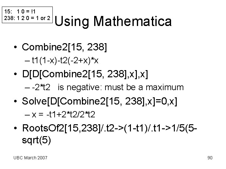
15: 1 0 = !1 238: 1 2 0 = 1 or 2 Using Mathematica • Combine 2[15, 238] – t 1(1 -x)-t 2(-2+x)*x • D[D[Combine 2[15, 238], x] – -2*t 2 is negative: must be a maximum • Solve[D[Combine 2[15, 238], x]=0, x] – x = -t 1+2*t 2/2*t 2 • Roots. Of 2[15, 238]/. t 2 ->(1 -t 1)/. t 1 ->1/5(5 sqrt(5) UBC March 2007 90

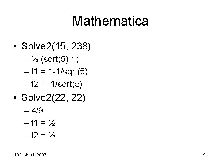
Mathematica • Solve 2(15, 238) – ½ (sqrt(5)-1) – t 1 = 1 -1/sqrt(5) – t 2 = 1/sqrt(5) • Solve 2(22, 22) – 4/9 – t 1 = ½ – t 2 = ½ UBC March 2007 91

Mathematica Include. It[r_, n_] : = Mod[Floor[r/n], 2]; App. SAT[r_] : = Simplify[Include. It[r, 1]*x^0*((1 - x))^((3 - 0)) + (( Include. It[r, 2] + Include. It[r, 4] + Include. It[r, 16]))* x^1*((1 - x))^((3 - 1)) + ((Include. It[r, 8] + Include. It[r, 32] + Include. It[r, 64]))* x^2*((1 - x))^((3 - 2)) + Include. It[r, 128]*x^3*((1 - x))^((3 - 3))]; Combine 2[r 1_, r 2_] : = t 1*App. SAT[r 1] + t 2*App. SAT[r 2]; Roots. Of 2[r 1_, r 2_] : = Replace. All[Combine 2[r 1, r 2], Solve[D[Combine 2[r 1, r 2], x] == 0, x]]; Solve 2[r 1_, r 2_] : = For [i = 1, i <= Length[ Roots. Of 2[r 1, r 2]], i++, Print[Minimize[{ Roots. Of 2[r 1, r 2][[ i]], 0 < t 1 < 1, 0 < t 2 < 1, t 1 + t 2 == 1}, {t 1, t 2}]]]; UBC March 2007 92