The EM algorithm Part 1 LING 572 Fei

The EM algorithm (Part 1) LING 572 Fei Xia 02/23/06

What is EM? • EM stands for “expectation maximization”. • A parameter estimation method: it falls into the general framework of maximum-likelihood estimation (MLE). • The general form was given in (Dempster, Laird, and Rubin, 1977), although essence of the algorithm appeared previously in various forms.

Outline • MLE • EM: basic concepts

MLE

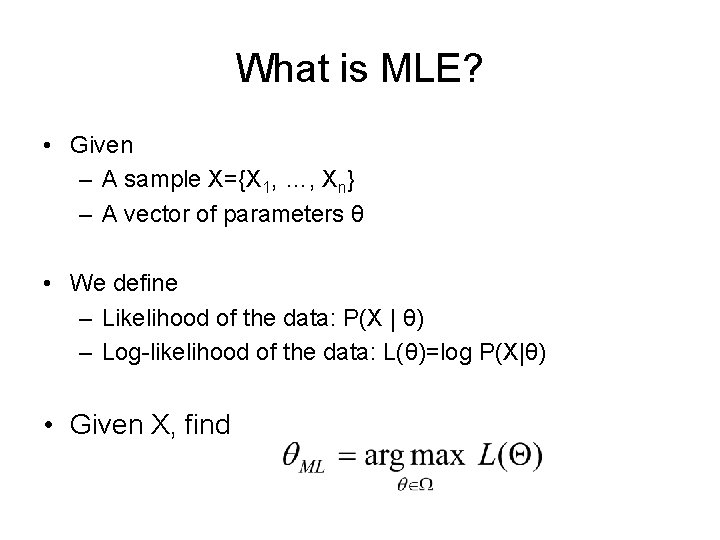
What is MLE? • Given – A sample X={X 1, …, Xn} – A vector of parameters θ • We define – Likelihood of the data: P(X | θ) – Log-likelihood of the data: L(θ)=log P(X|θ) • Given X, find

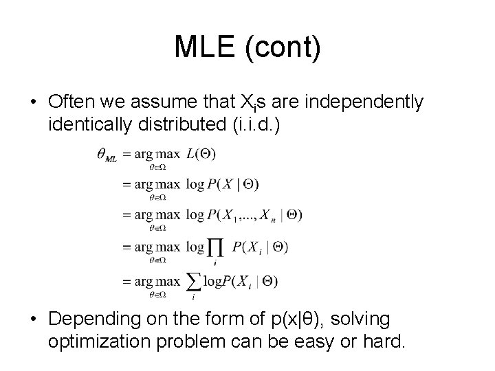
MLE (cont) • Often we assume that Xis are independently identically distributed (i. i. d. ) • Depending on the form of p(x|θ), solving optimization problem can be easy or hard.

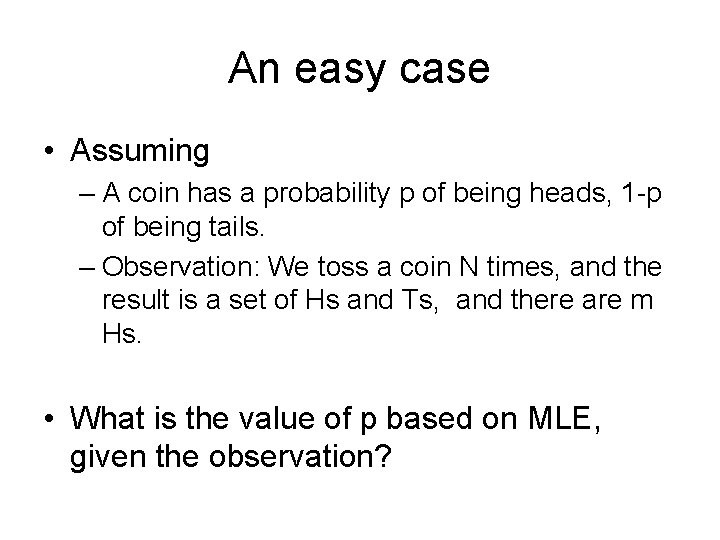
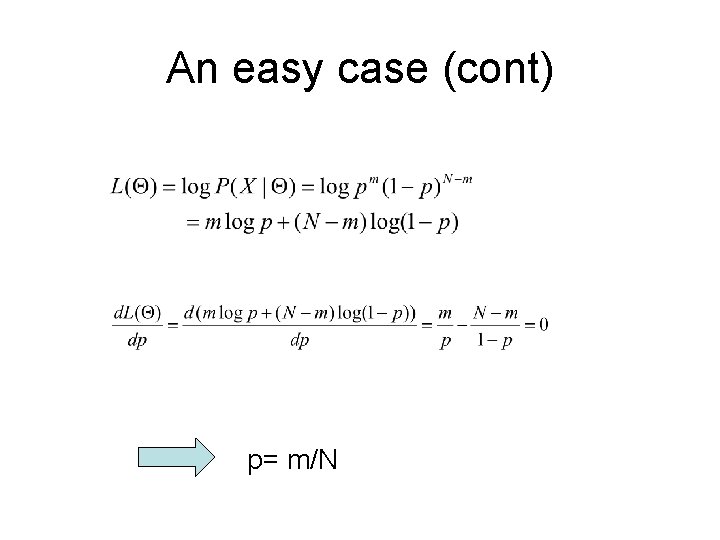
An easy case • Assuming – A coin has a probability p of being heads, 1 -p of being tails. – Observation: We toss a coin N times, and the result is a set of Hs and Ts, and there are m Hs. • What is the value of p based on MLE, given the observation?

An easy case (cont) p= m/N

EM: basic concepts

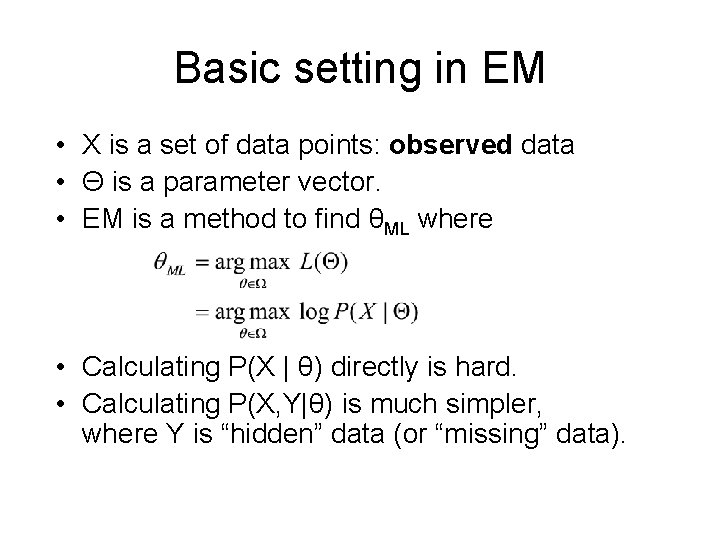
Basic setting in EM • X is a set of data points: observed data • Θ is a parameter vector. • EM is a method to find θML where • Calculating P(X | θ) directly is hard. • Calculating P(X, Y|θ) is much simpler, where Y is “hidden” data (or “missing” data).

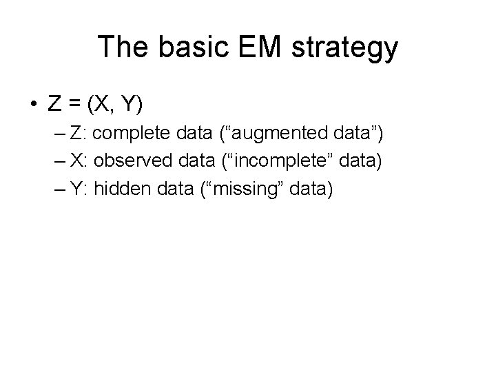
The basic EM strategy • Z = (X, Y) – Z: complete data (“augmented data”) – X: observed data (“incomplete” data) – Y: hidden data (“missing” data)

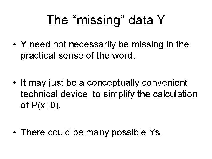
The “missing” data Y • Y need not necessarily be missing in the practical sense of the word. • It may just be a conceptually convenient technical device to simplify the calculation of P(x |θ). • There could be many possible Ys.

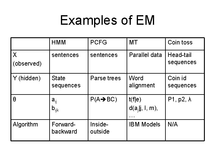
Examples of EM HMM PCFG MT Coin toss X (observed) sentences Parallel data Head-tail sequences Y (hidden) State sequences Parse trees Word alignment Coin id sequences θ aij bijk P(A BC) t(f|e) d(aj|j, l, m), … P 1, p 2, λ Algorithm Forwardbackward Insideoutside IBM Models N/A

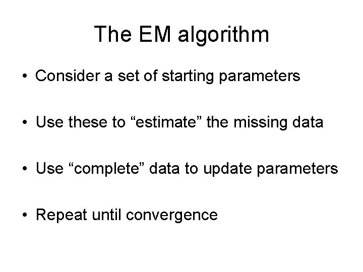
The EM algorithm • Consider a set of starting parameters • Use these to “estimate” the missing data • Use “complete” data to update parameters • Repeat until convergence

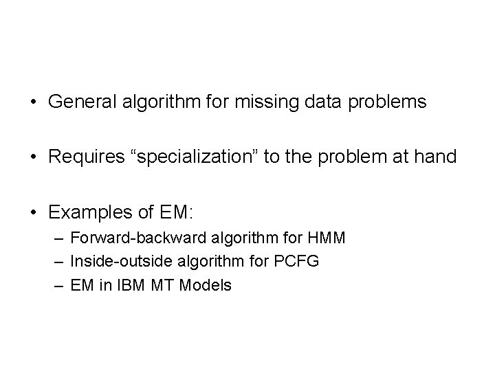
• General algorithm for missing data problems • Requires “specialization” to the problem at hand • Examples of EM: – Forward-backward algorithm for HMM – Inside-outside algorithm for PCFG – EM in IBM MT Models

Strengths of EM • Numerical stability: in every iteration of the EM algorithm, it increases the likelihood of the observed data. • The EM handles parameter constraints gracefully.

Problems with EM • Convergence can be very slow on some problems and is intimately related to the amount of missing information. • It guarantees to improve the probability of the training corpus, which is different from reducing the errors directly. • It cannot guarantee to reach global maximum (it could get struck at the local maxima, saddle points, etc) The initial values are important.

Additional slides

Setting for the EM algorithm • Problem is simpler to solve for complete data – Maximum likelihood estimates can be calculated using standard methods. • Estimates of mixture parameters could be obtained in straightforward manner if the origin of each observation is known.

EM algorithm for mixtures • “Guesstimate” starting parameters • E-step: Use Bayes’ theorem to calculate group assignment probabilities • M-step: Update parameters using estimated assignments • Repeat steps 2 and 3 until likelihood is stable.

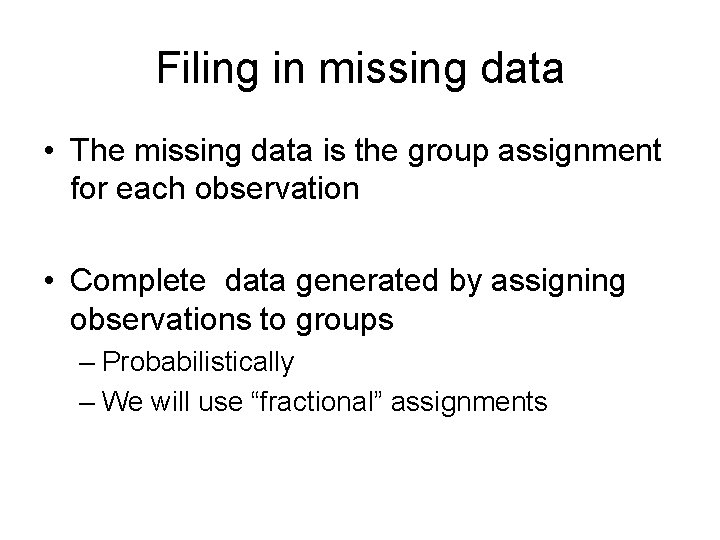
Filing in missing data • The missing data is the group assignment for each observation • Complete data generated by assigning observations to groups – Probabilistically – We will use “fractional” assignments

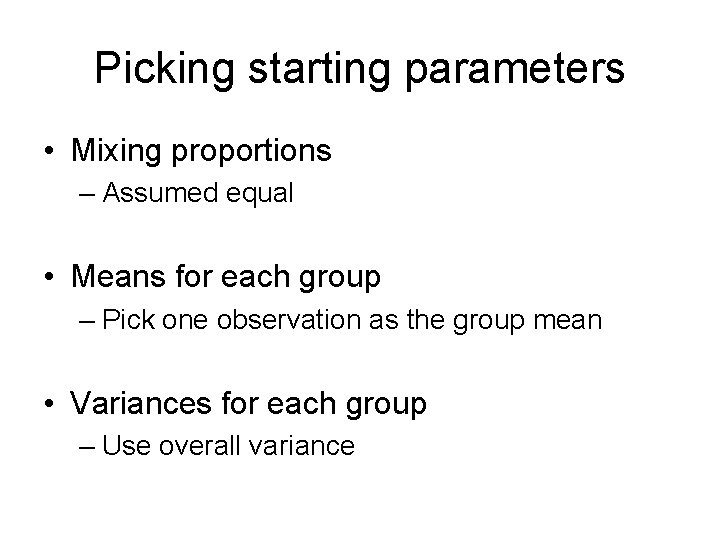
Picking starting parameters • Mixing proportions – Assumed equal • Means for each group – Pick one observation as the group mean • Variances for each group – Use overall variance