THE ECONOMICS OF ENVIRONMENTAL QUALITY Field chapter 5

THE ECONOMICS OF ENVIRONMENTAL QUALITY Field, chapter 5

Introduction n Chapter 5 is probably the key chapter in the book in terms of conceptual matters. q q The market system, left to itself, is likely to malfunction when matters of environmental pollution are involved. This brings us to the policy question: If we do not like the way things are currently turning out, what steps should be undertaken to change the situation?

Policy Questions n The policy problem includes a number of closely related issues. q q One of the first is that of identifying the most appropriate level of environmental quality we ought to try to achieve. Another is how to divide up the task of meeting environmental quality goals. n If we have many polluters, how should we seek to allocate among them an overall reduction in emissions?

A Simplified Model n Diverse types of environmental pollutants call for diverse types of public policy. n To build up the required policy analyses it is better to start with one very simple model that lays out the fundamentals of the policy situation.

Trade-Offs n The essence of the model consists of a simple trade-off situation that characterizes all pollution-control activities. q q Reducing emissions reduces the damages that people suffer from environmental pollution But reducing emissions takes resources that could have been used in some other way. n Suggests that optimal level of pollution is not zero.

Damages n Consider a simple situation where a firm (e. g. , a pulp mill) is emitting production residuals into a river. q q As these residuals are carried downstream, they tend to be transformed into less damaging chemical constituents, but before that process is completed the river passes by a large metropolitan area. One side of the trade-off is the damages that people experience when the environment is degraded.

Abatement n The offending pulp mill could reduce the amount of effluent by treating its wastes before discharge. q q This act of reducing, or abating, some portion of its wastes will require resources, the costs of which will affect the price of the paper it produces. These abatement costs are the other side of the basic pollution-control trade-off.

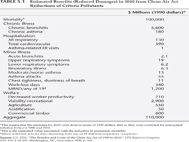
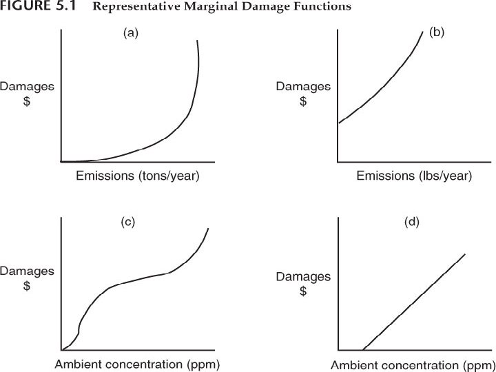
POLLUTION DAMAGES n n By damages we mean all the negative impacts that users of the environment experience as a result of the degradation of that environment. In general, the greater the pollution, the greater the damages it produces. q To describe the relationship between pollution and damage, we will use the idea of a damage function.

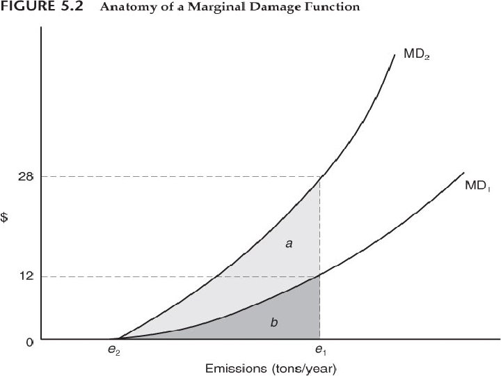
Damage Functions: A Closer Look n n Figure 5 -2 shows two marginal emissions damage functions. It is important to remember that these are time specific. q q They show the emissions and the marginal damages for a particular period of time. For purposes of simplicity, the graph refers to a strictly noncumulative pollutant. n All damages occur in the same period as emissions.

ABATEMENT COSTS n Abatement costs are the costs of reducing the quantity of residuals being emitted into the environment, or of lowering ambient concentrations. q Abatement costs normally will differ from one source to another, depending on a variety of factors. n The costs of reducing emissions of SO 2 from electric power plants will be different from the costs of reducing toxic fumes from chemical plants.

Abatement Costs (cont’d) n Even for sources producing the same type of effluent the costs of abatement are likely to be different. q Differences in the technological features n n One source may be relatively new, using modern production technology Another may be an old one using more highly polluting technology.

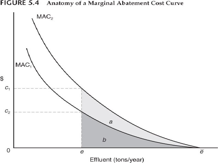
Abatement Cost Functions n n n On the horizontal axis, marginal abatement cost curves originate at the uncontrolled emission levels, ē. From this origin point, marginal abatement costs show the marginal costs of producing reductions in emissions. Thus, these marginal cost curves rise from right to left, depicting rising marginal costs of reducing emissions.

Rising Marginal Abatement Costs n Think again of the pulp mill. q q This first small decrease in pollution might be obtained with the addition of a modest settling pond. To get a 30 -40 percent reduction, the pulp mill may have to invest in new technology that is more efficient in terms of water use.

Marginal Abatement Costs n Differences between MAC 1 and MAC 2 ? q q The newer plant lends itself to less costly emissions reduction. Different times. n Before and after a technological change.

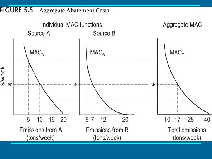
Aggregate Marginal Abatement Costs n The aggregate marginal abatement cost curve is a summation, or aggregation, of individual relationships. q The total cost will depend on how the total emissions are allocated among the different sources. n n Add together the individual functions to yield the lowest possible aggregate marginal abatement costs. The way to do this is to add them horizontally.

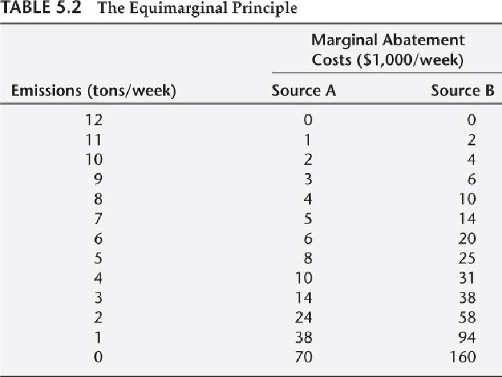
Equimarginal Principle n n In effect what we have done here is to invoke the important equimarginal principle. To get the minimum aggregate marginal abatement cost curve, the aggregate level of emissions must be distributed among the different sources in such a way that they all have the same marginal abatement costs.

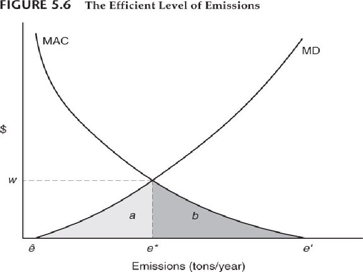
THE SOCIALLY EFFICIENT LEVEL OF EMISSIONS n n The "efficient" level of emissions is defined as that level at which marginal damages are equal to marginal abatement costs. What is the justification for this? q A trade-off is inherent… n n Higher emissions expose society to greater costs stemming from environmental damages. Lower emissions mean greater costs in the form of resources devoted to abatement activities.

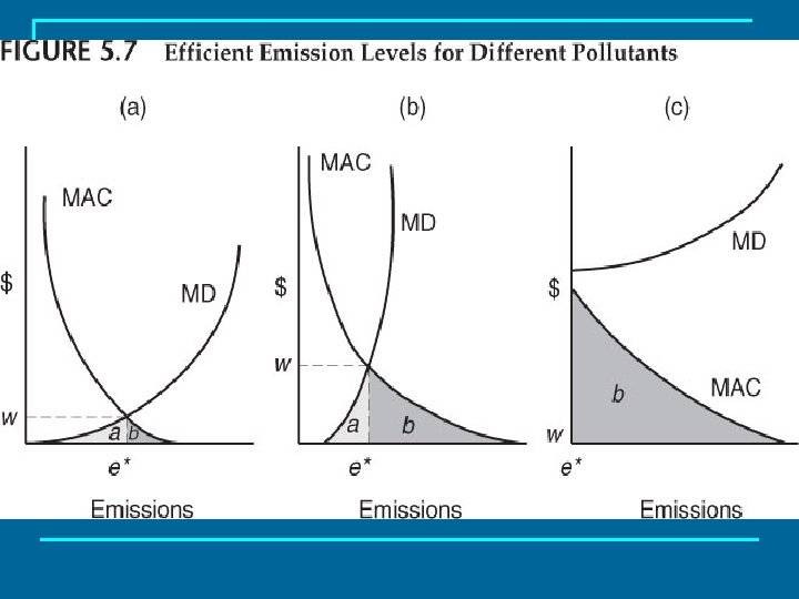
Does e* Mean High Emissions? n n e* might suggest that the "efficient" level of emissions is always one that involves a relatively large quantity of emissions and substantial environmental damages. This is not the case. q q What we are developing, rather, is a conceptual way of looking at a trade-off. In the real world every pollution problem is different.

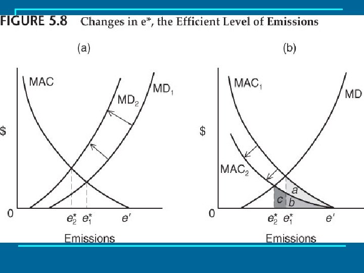
Changes In the Efficient Level of Emissions n n The level of emissions that was efficient last year, or last decade, is not necessarily the level that is efficient today or that is likely to be in the future. When any of the factors that lie behind the marginal damage and marginal abatement cost functions change, the functions will shift and e* will change.

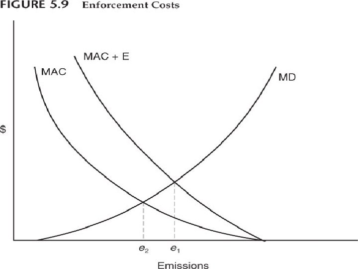
ENFORCEMENT COSTS n n Emission reductions do not happen unless resources are devoted to enforcement. To include all sources of cost we need to add enforcement costs to the analysis. q Some of these are private, such as added recordkeeping by polluters, but the bulk are public costs related to various regulatory aspects of the enforcement process.

Enforcement Costs n n The addition of enforcement costs moves the efficient level of emissions to the right of where it would be if they were zero. This shows the vital importance of having good enforcement technology because lower marginal enforcement costs would move MAC + E closer to MAC, decreasing the efficient emission level.

THE EQUIMARGINAL PRINCIPLE APPLIED TO EMISSION REDUCTIONS n The application of the equimarginal principle says the following: If there are multiple sources of a particular type of pollutant with differing marginal abatement costs, and if it is desired to reduce aggregate emissions at the least possible cost (or alternatively, get the greatest reduction in emissions for a given cost), then emissions from the various sources must be reduced in accordance with the equimarginal principle.

Equiproportionate n n If Source A were cut 50 percent to 6 tons/week, its MAC at this level would be $6, 000/week, whereas at this level of emissions the MAC of Source B would be $20, 000/week. Total abatement costs of the 12 -ton total are $21, 000/week for Source A and $56, 000/week for Source B or a grand total of $77, 000/week.

Equimarginal n n A and B must have different emission rates but together emit no more than 12 tons of effluent and have the same marginal abatement costs. This condition is satisfied if Source A emits 4 tons and Source B emits 8 tons. These rates add up to 12 tons total and give each source a marginal abatement cost of $10, 000/week. q q q TAC = $39, 000/week for Source A TAC = $22, 000/week for Source B TAC = $61, 000/week grand total.

Summary n The model is very general and risks giving an overly simplistic impression of pollution problems in the real world. q n Few actual instances where the marginal damage and marginal abatement functions are known with certainty. The simple model is useful for thinking about the basic problem of pollution control. q It will be useful in our later chapters on the various approaches to environmental policy.