The Demand Curves Graphical Derivation We start with

The Demand Curves Graphical Derivation

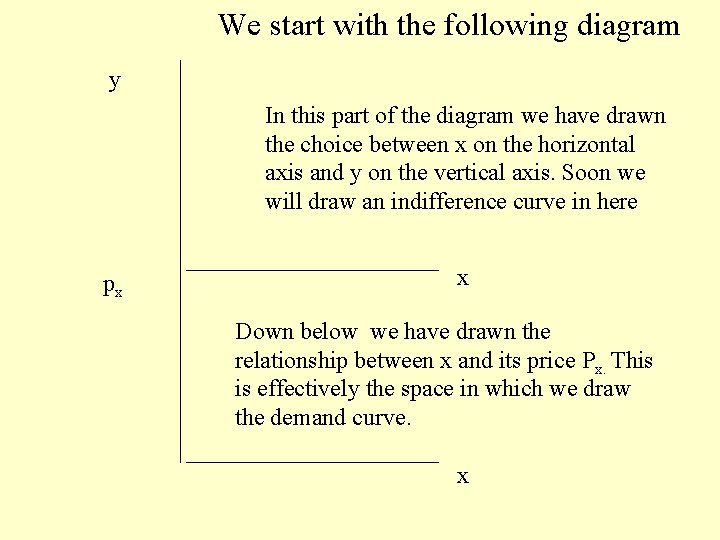
We start with the following diagram y In this part of the diagram we have drawn the choice between x on the horizontal axis and y on the vertical axis. Soon we will draw an indifference curve in here px x Down below we have drawn the relationship between x and its price Px. This is effectively the space in which we draw the demand curve. x

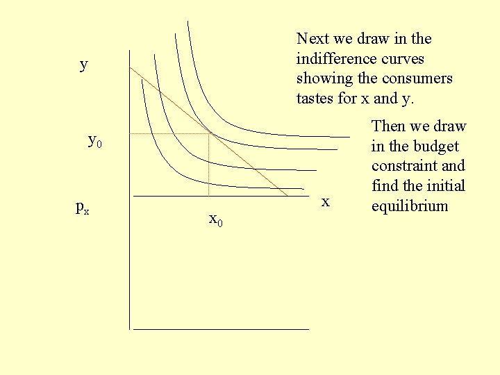
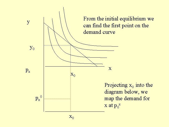
Next we draw in the indifference curves showing the consumers tastes for x and y. y y 0 px x 0 x Then we draw in the budget constraint and find the initial equilibrium

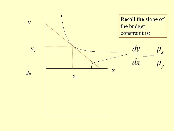
Recall the slope of the budget constraint is: y y 0 px x 0 x

From the initial equilibrium we can find the first point on the demand curve y y 0 px x 0 x Projecting x 0 into the diagram below, we map the demand for x at p 0 x px 0

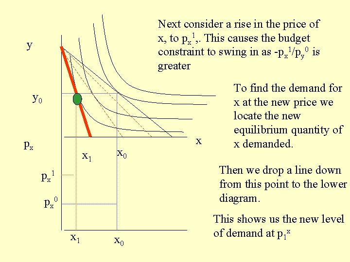
Next consider a rise in the price of x, to px 1, . This causes the budget constraint to swing in as -px 1/py 0 is greater y y 0 px x 1 x 0 x To find the demand for x at the new price we locate the new equilibrium quantity of x demanded. Then we drop a line down from this point to the lower diagram. px 1 px 0 x 1 x 0 This shows us the new level of demand at p 1 x

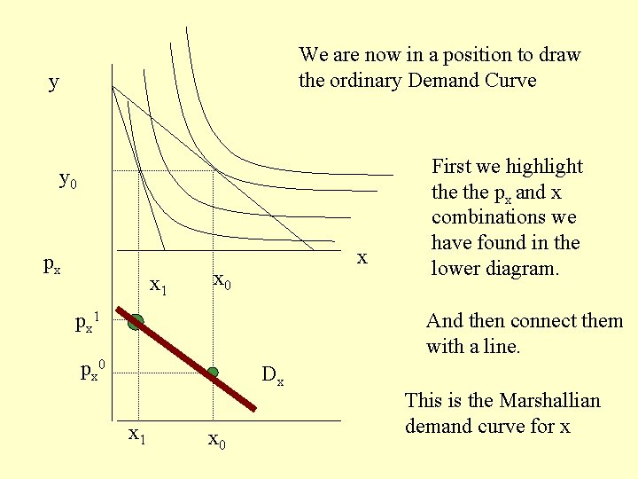
We are now in a position to draw the ordinary Demand Curve y y 0 px x 1 x x 0 px 1 First we highlight the px and x combinations we have found in the lower diagram. And then connect them with a line. px 0 Dx x 1 x 0 This is the Marshallian demand curve for x

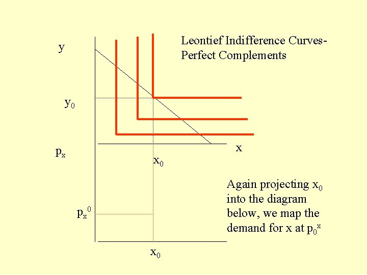
• In the diagrams above we have drawn our demand curve as a nice downward sloping curve. • Will this always be the case? • Consider the case of perfect Complements (Leontief Indifference Curve) e. g. Left and Right Shoes

Leontief Indifference Curves. Perfect Complements y y 0 px x 0 x Again projecting x 0 into the diagram below, we map the demand for x at p 0 x px 0

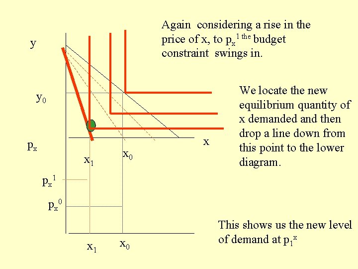
Again considering a rise in the price of x, to px 1 the budget constraint swings in. y y 0 px x 1 x 0 x We locate the new equilibrium quantity of x demanded and then drop a line down from this point to the lower diagram. px 1 px 0 x 1 x 0 This shows us the new level of demand at p 1 x

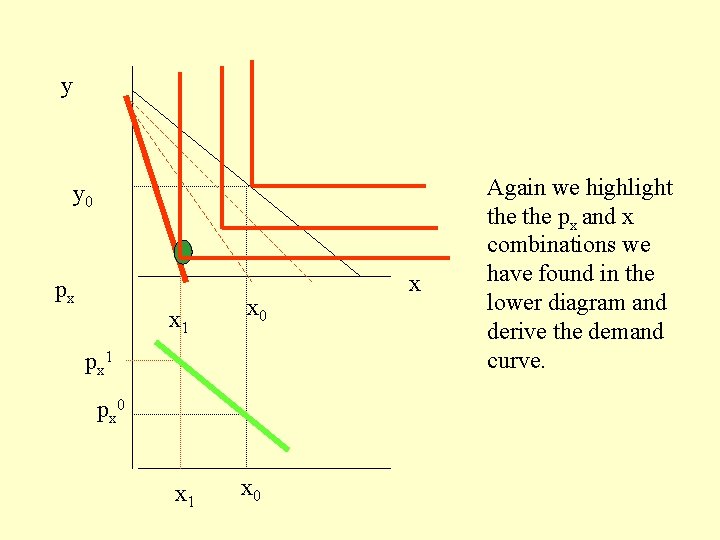
y y 0 px x 1 x 0 px 1 px 0 x Again we highlight the px and x combinations we have found in the lower diagram and derive the demand curve.

• In the diagrams above we have drawn our demand curve as a nice downward sloping curve. • Will this always be the case? • Consider the case of perfect Complements (Leontief Indifference Curve) e. g. Left and Right Shoes

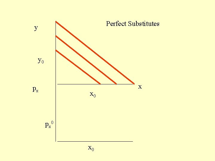
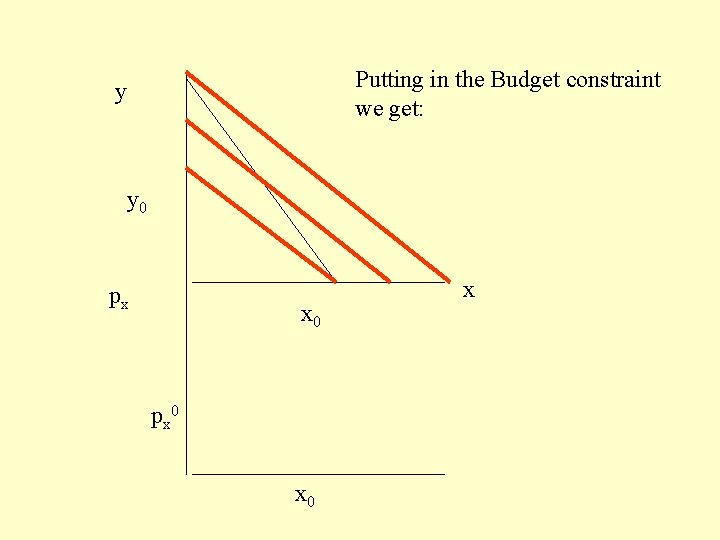
Perfect Substitutes y y 0 px x 0 px 0 x

Putting in the Budget constraint we get: y y 0 px x 0 px 0 x

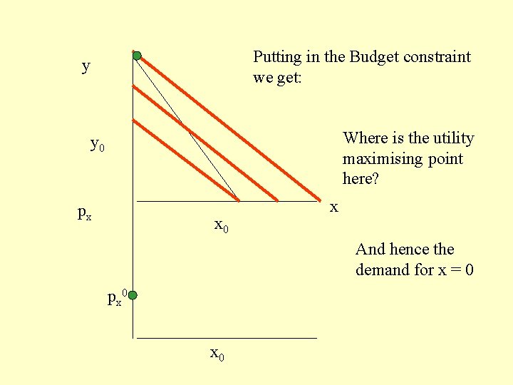
Putting in the Budget constraint we get: y Where is the utility maximising point here? y 0 px x 0 x And hence the demand for x = 0 px 0

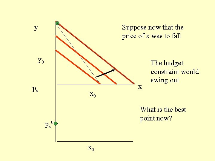
y Suppose now that the price of x was to fall y 0 px x 0 x The budget constraint would swing out What is the best point now? px 0

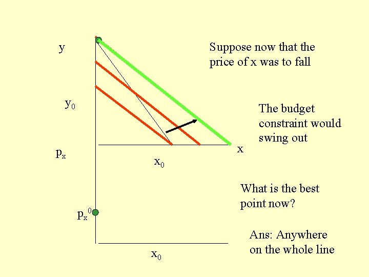
y Suppose now that the price of x was to fall y 0 px x 0 x The budget constraint would swing out What is the best point now? px 0 Ans: Anywhere on the whole line

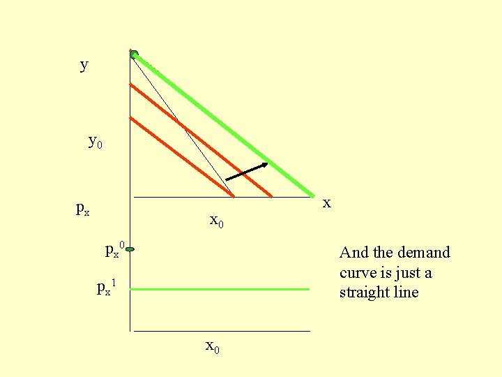
y y 0 px x 0 px 0 x And the demand curve is just a straight line px 1 x 0

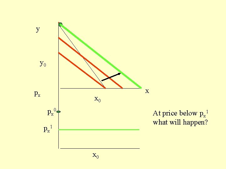
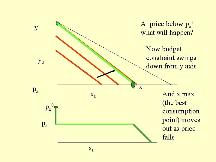
y y 0 px x 0 px 0 x At price below px 1 what will happen? px 1 x 0

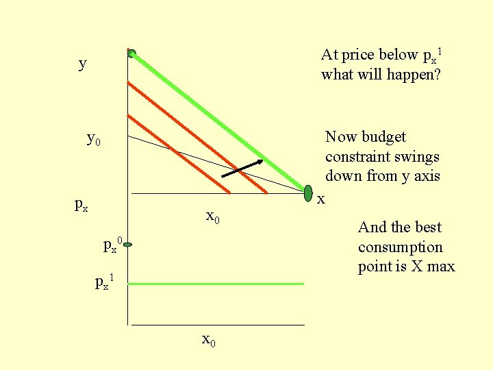
At price below px 1 what will happen? y y 0 Now budget constraint swings down from y axis px x 0 px 1 x 0 x And the best consumption point is X max

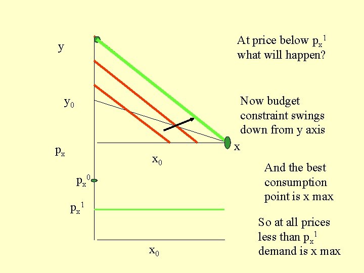
At price below px 1 what will happen? y y 0 Now budget constraint swings down from y axis px x 0 px 1 x 0 x And the best consumption point is x max So at all prices less than px 1 demand is x max

At price below px 1 what will happen? y Now budget constraint swings down from y axis y 0 px x 0 px 1 x 0 x And x max (the best consumption point) moves out as price falls

• So here the demand curve does not take the usual nice smooth downward sloping shape. • What determines the shape of the demand curve • Ans: The shape of the indifference curves. • Q: What properties must indifference curve have to give us sensible looking demand curves