The Cover Time of Random Walks Uriel Feige

The Cover Time of Random Walks Uriel Feige Weizmann Institute

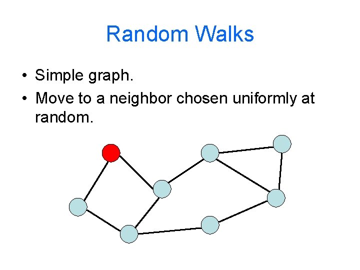
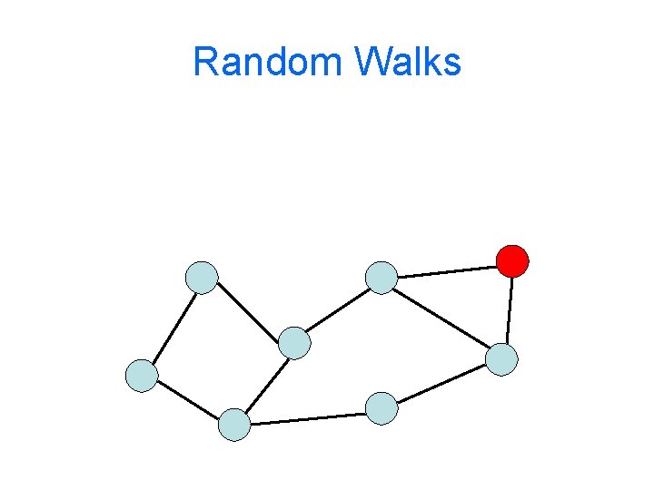
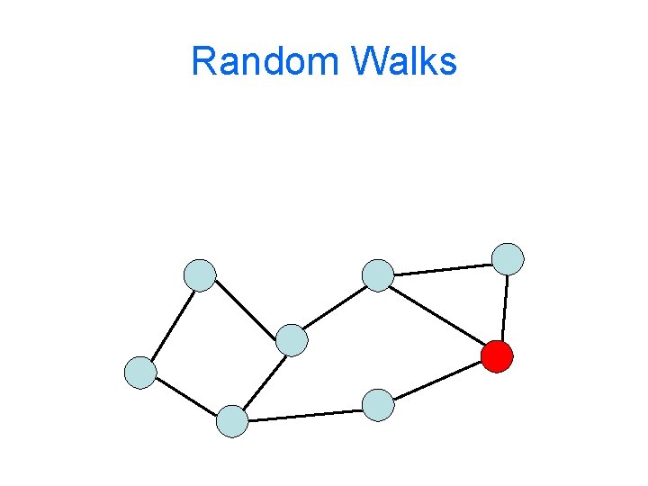
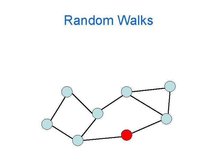
Random Walks • Simple graph. • Move to a neighbor chosen uniformly at random.

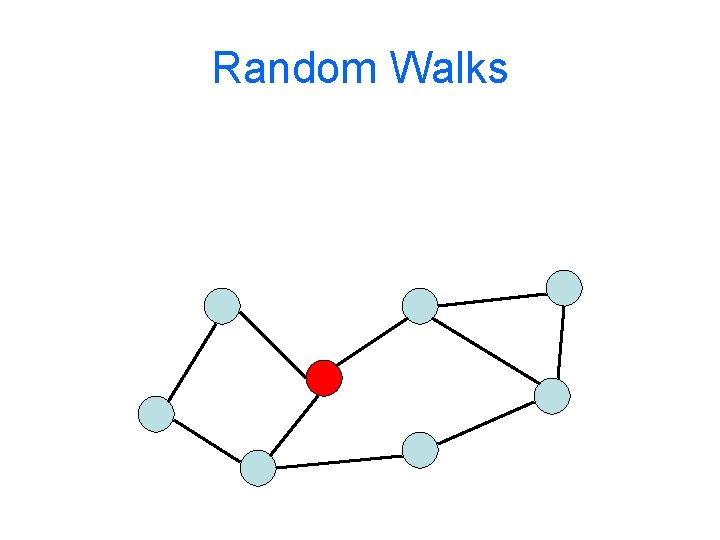
Random Walks

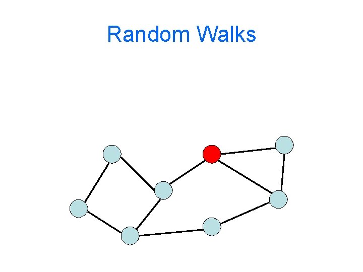
Random Walks

Random Walks

Random Walks

Random Walks

Random Walks

Random Walks

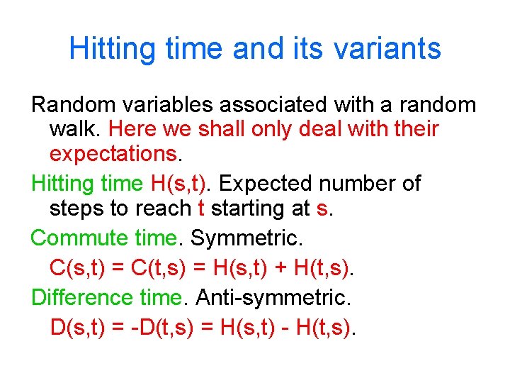
Hitting time and its variants Random variables associated with a random walk. Here we shall only deal with their expectations. Hitting time H(s, t). Expected number of steps to reach t starting at s. Commute time. Symmetric. C(s, t) = C(t, s) = H(s, t) + H(t, s). Difference time. Anti-symmetric. D(s, t) = -D(t, s) = H(s, t) - H(t, s).

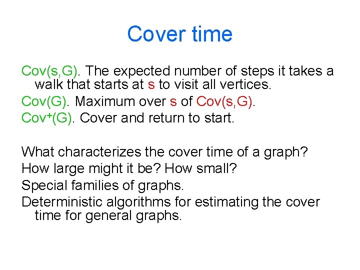
Cover time Cov(s, G). The expected number of steps it takes a walk that starts at s to visit all vertices. Cov(G). Maximum over s of Cov(s, G). Cov+(G). Cover and return to start. What characterizes the cover time of a graph? How large might it be? How small? Special families of graphs. Deterministic algorithms for estimating the cover time for general graphs.

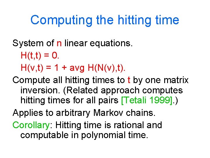
Computing the hitting time System of n linear equations. H(t, t) = 0. H(v, t) = 1 + avg H(N(v), t). Compute all hitting times to t by one matrix inversion. (Related approach computes hitting times for all pairs [Tetali 1999]. ) Applies to arbitrary Markov chains. Corollary: Hitting time is rational and computable in polynomial time.

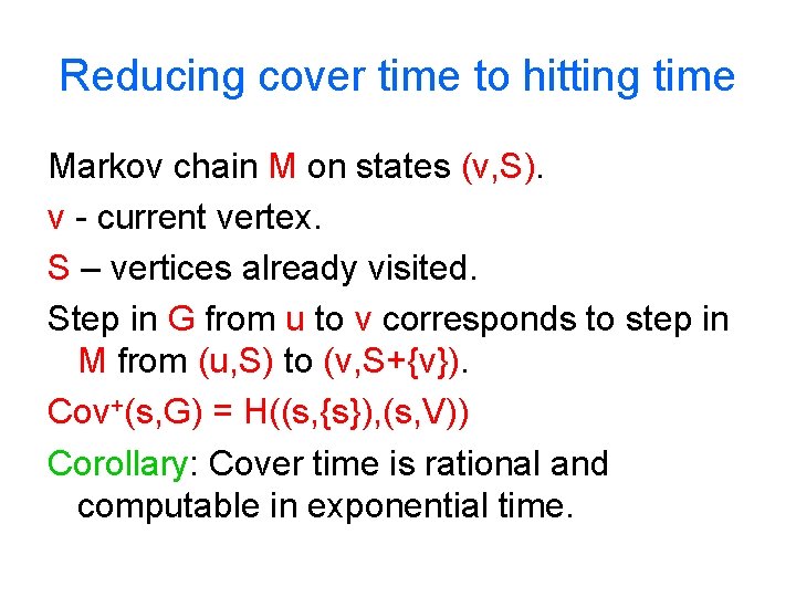
Reducing cover time to hitting time Markov chain M on states (v, S). v - current vertex. S – vertices already visited. Step in G from u to v corresponds to step in M from (u, S) to (v, S+{v}). Cov+(s, G) = H((s, {s}), (s, V)) Corollary: Cover time is rational and computable in exponential time.

A detour - electrical networks Many analogies between random walks in graphs and electrical networks. Can help (depending on a person’s background) in transferring intuition and theorems from one area to the other.

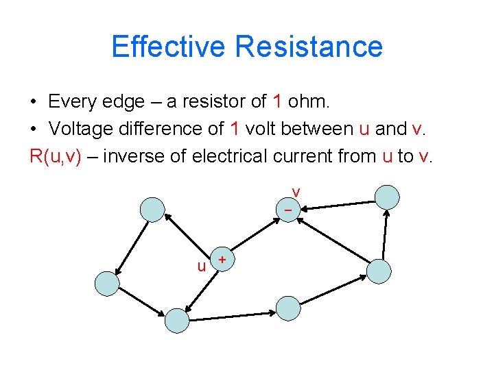
Effective Resistance • Every edge – a resistor of 1 ohm. • Voltage difference of 1 volt between u and v. R(u, v) – inverse of electrical current from u to v. _ u + v

Understanding the commute time Theorem [Chandra, Raghavan, Ruzzo, Smolensky, Tiwari 1989]: For every graph with m edges and every two vertices u and v, C(u, v) = 2 m. R(u, v) Proof: by comparing the respective systems of linear equations, for random walks and for electrical current flows.

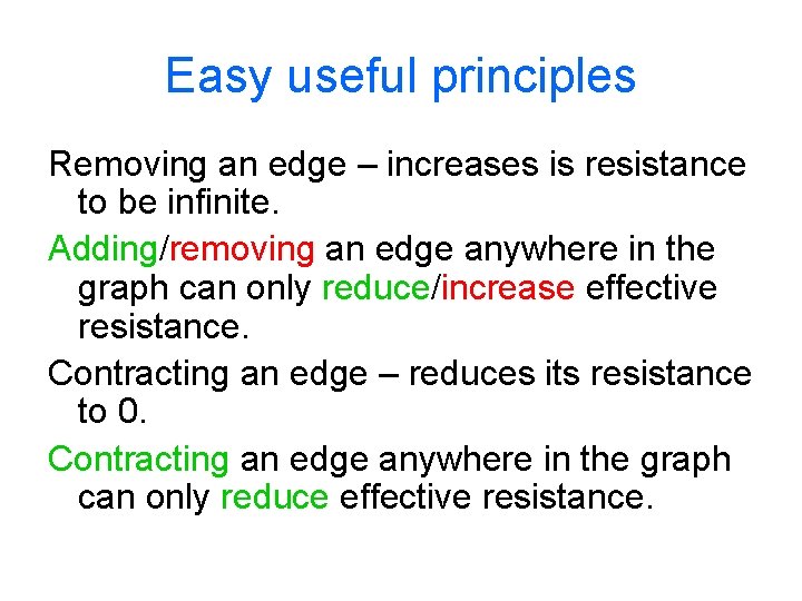
Easy useful principles Removing an edge – increases is resistance to be infinite. Adding/removing an edge anywhere in the graph can only reduce/increase effective resistance. Contracting an edge – reduces its resistance to 0. Contracting an edge anywhere in the graph can only reduce effective resistance.

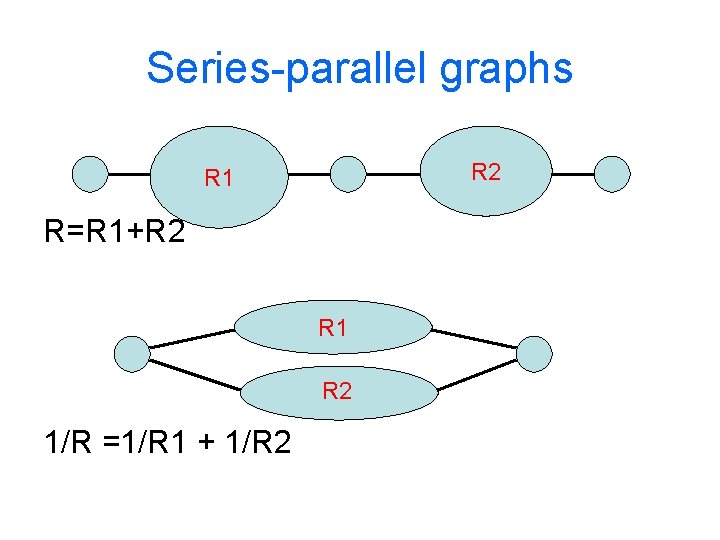
Series-parallel graphs R 2 R 1 R=R 1+R 2 R 1 R 2 1/R =1/R 1 + 1/R 2

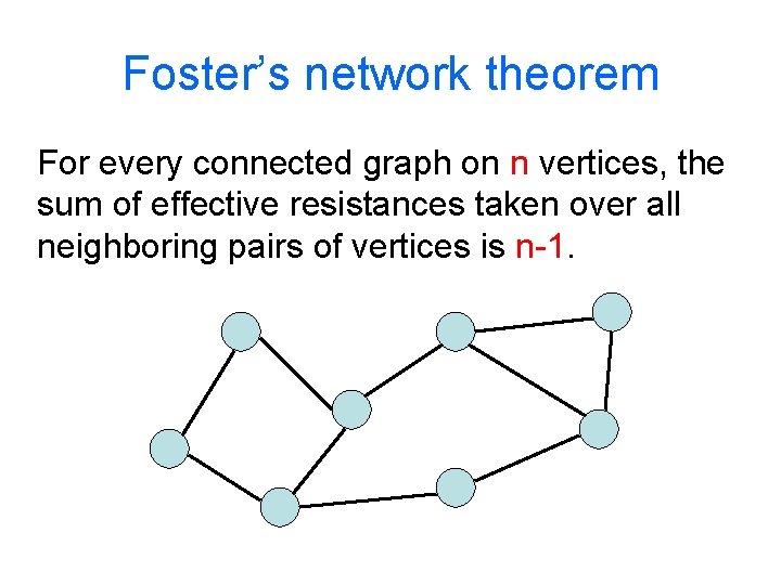
Foster’s network theorem For every connected graph on n vertices, the sum of effective resistances taken over all neighboring pairs of vertices is n-1.

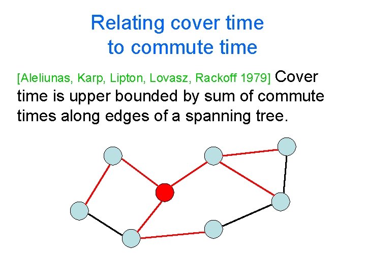
Relating cover time to commute time Cover time is upper bounded by sum of commute times along edges of a spanning tree. [Aleliunas, Karp, Lipton, Lovasz, Rackoff 1979]

Spanning tree argument Arbitrary spanning tree [AKLLR, CRRST]: Best spanning tree [Feige 1995]: Lollipop graph: n/3 path 2 n/3 clique

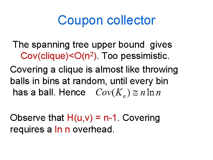
Coupon collector The spanning tree upper bound gives Cov(clique)<O(n 2). Too pessimistic. Covering a clique is almost like throwing balls in bins at random, until every bin has a ball. Hence Observe that H(u, v) = n-1. Covering requires a ln n overhead.

Relating cover time to hitting time [Matthews 1988] nth harmonic number

Proof of Matthews bound Arbitrarily order all vertices but s. Let Pr[i] denote the probability that i is the last vertex to be visited among {1, …, i}. For random permutation, Pr[i] = 1/i.

Lower bound on cover time [Feige 1995]: Proof: eithere is a pair of vertices that witness the lower bound through their mutual hitting times, or a generalization of the Matthew’s bound (applying it to subsets of vertices) works.

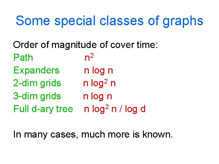
Some special classes of graphs Order of magnitude of cover time: Path n 2 Expanders n log n 2 -dim grids n log 2 n 3 -dim grids n log n Full d-ary tree n log 2 n / log d In many cases, much more is known.

Regularity and cover time [Kahn, Linial, Nisan, Saks 1989]: the cover time on regular graphs is at most 4 n 2. [Coppersmith, Feige, Shearer 1996]: every spanning tree has resistance at most 3 n/d. [Feige 1997]: cover time at most 2 n 2. Worse example known (necklace): 15 n 2/16.

Irregular graphs [Coppersmith, Feige, Shearer 1996]: every graph has a spanning tree of resistance at most O(n avg(1/deg)). Proof: random spanning tree. Uses the fact that fraction of spanning trees that use edge (u, v) is exactly R[u, v]. Upper bound on Cov+(G) based on irregularity avg(deg) x avg(1/deg) of G.

Spanning tree - without return [Feige 1997] (proof essentially, by induction): • In every graph there is a vertex s with • Path is the most difficult tree to cover (starting at the middle).

Approximating Cov(G) Max[C(u, v)] approximates Cov(G) within a factor of log n. Augmented Matthews lower bound (AMLB): [Kahn, Kim, Lovasz, Vu 2000]: AMLB approximated Cov(G) within a factor of O((log n)2), and can be efficiently approximated within a factor of 2.

Approximating Cov(s, G) might be much larger than max[H(s, v)]. key graph [Chlamtac, Feige, Rabinovich 2003, 2005]: Cov(s, G) can be approximated within a ratio of O(log n approx[Cov(G)]).

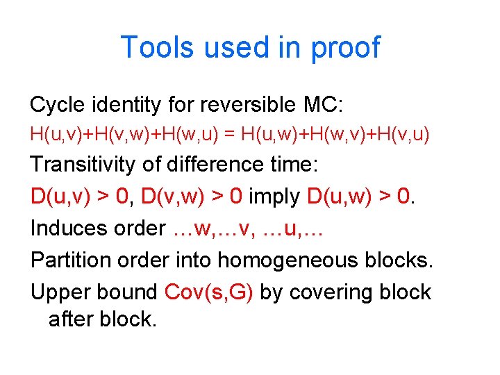
Tools used in proof Cycle identity for reversible MC: H(u, v)+H(v, w)+H(w, u) = H(u, w)+H(w, v)+H(v, u) Transitivity of difference time: D(u, v) > 0, D(v, w) > 0 imply D(u, w) > 0. Induces order …w, …v, …u, … Partition order into homogeneous blocks. Upper bound Cov(s, G) by covering block after block.

Full d-ary trees Cover time known in great detail [Aldous]. The technique: Compute return time to root r (easy). Compute expected number of returns to root during cover (recursive formula). Multiply the two to get Cov+(r, T).

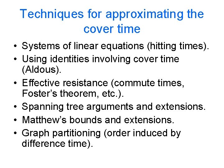
Techniques for approximating the cover time • Systems of linear equations (hitting times). • Using identities involving cover time (Aldous). • Effective resistance (commute times, Foster’s theorem, etc. ). • Spanning tree arguments and extensions. • Matthew’s bounds and extensions. • Graph partitioning (order induced by difference time).

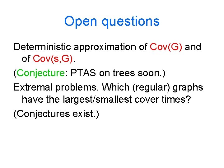
Open questions Deterministic approximation of Cov(G) and of Cov(s, G). (Conjecture: PTAS on trees soon. ) Extremal problems. Which (regular) graphs have the largest/smallest cover times? (Conjectures exist. )

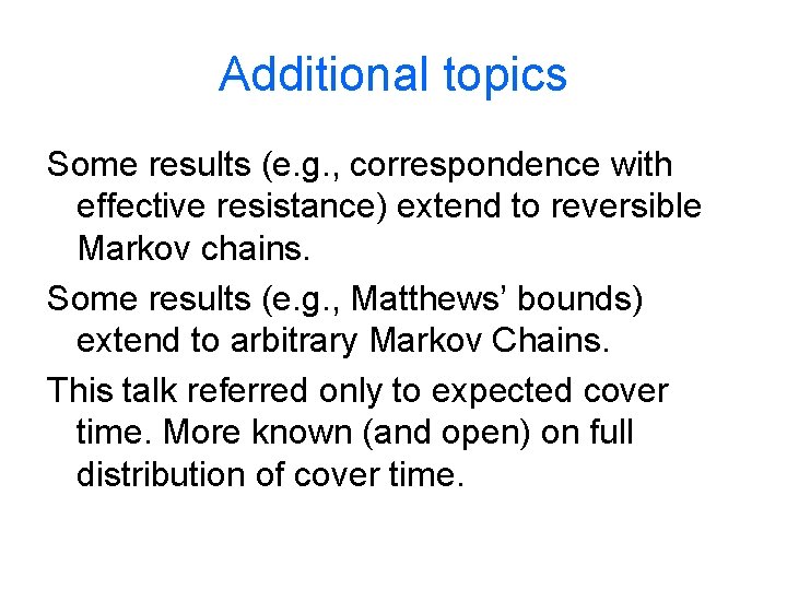
Additional topics Some results (e. g. , correspondence with effective resistance) extend to reversible Markov chains. Some results (e. g. , Matthews’ bounds) extend to arbitrary Markov Chains. This talk referred only to expected cover time. More known (and open) on full distribution of cover time.