THE COSTS OF PRODUCTION 0 Chapter 13 The

THE COSTS OF PRODUCTION 0

Chapter 13: The Costs of Production Econ 2100 THE COSTS OF PRODUCTION 1

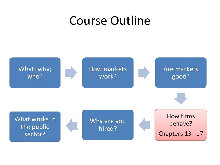
Course Outline What; why; who? What works in the public sector? How markets work? Are markets good? Why are you hired? How firms behave? Chapters 13 - 17

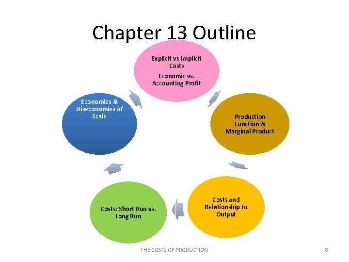
Chapter 13 Outline Explicit vs Implicit Costs Economic vs. Accounting Profit Economies & Diseconomies of Scale Production Function & Marginal Product Costs: Short Run vs. Long Run Costs and Relationship to Output THE COSTS OF PRODUCTION 3

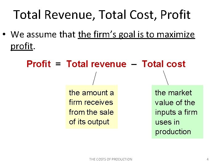
Total Revenue, Total Cost, Profit • We assume that the firm’s goal is to maximize profit. Profit = Total revenue – Total cost the amount a firm receives from the sale of its output THE COSTS OF PRODUCTION the market value of the inputs a firm uses in production 4

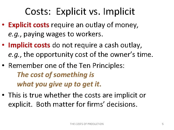
Costs: Explicit vs. Implicit • Explicit costs require an outlay of money, e. g. , paying wages to workers. • Implicit costs do not require a cash outlay, e. g. , the opportunity cost of the owner’s time. • Remember one of the Ten Principles: The cost of something is what you give up to get it. • This is true whether the costs are implicit or explicit. Both matter for firms’ decisions. THE COSTS OF PRODUCTION 5

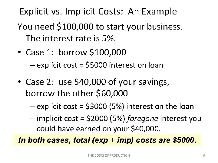
Explicit vs. Implicit Costs: An Example You need $100, 000 to start your business. The interest rate is 5%. • Case 1: borrow $100, 000 – explicit cost = $5000 interest on loan • Case 2: use $40, 000 of your savings, borrow the other $60, 000 – explicit cost = $3000 (5%) interest on the loan – implicit cost = $2000 (5%) foregone interest you could have earned on your $40, 000. In both cases, total (exp + imp) costs are $5000. THE COSTS OF PRODUCTION 6

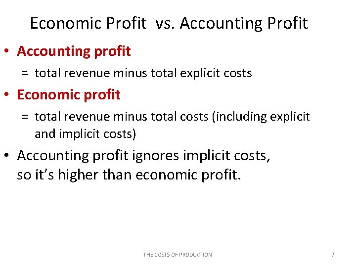
Economic Profit vs. Accounting Profit • Accounting profit = total revenue minus total explicit costs • Economic profit = total revenue minus total costs (including explicit and implicit costs) • Accounting profit ignores implicit costs, so it’s higher than economic profit. THE COSTS OF PRODUCTION 7

Chapter 13 Outline Explicit vs Implicit Costs Economic vs. Accounting Profit Economies & Diseconomies of Scale Production Function & Marginal Product Costs: Short Run vs. Long Run Costs and Relationship to Output THE COSTS OF PRODUCTION 8

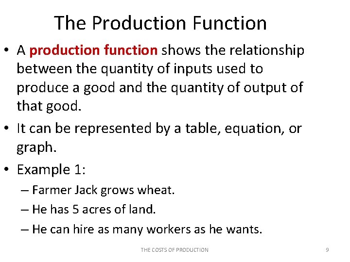
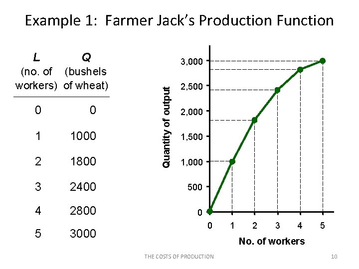
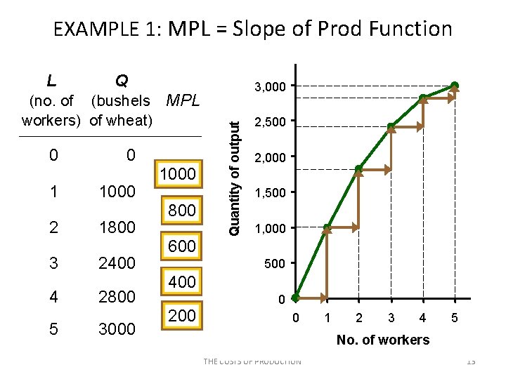
The Production Function • A production function shows the relationship between the quantity of inputs used to produce a good and the quantity of output of that good. • It can be represented by a table, equation, or graph. • Example 1: – Farmer Jack grows wheat. – He has 5 acres of land. – He can hire as many workers as he wants. THE COSTS OF PRODUCTION 9

Example 1: Farmer Jack’s Production Function Q (no. of (bushels workers) of wheat) 3, 000 Quantity of output L 2, 500 0 0 1 1000 2 1800 3 2400 500 4 2800 0 5 3000 2, 000 1, 500 1, 000 0 1 2 3 4 5 No. of workers THE COSTS OF PRODUCTION 10

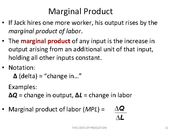
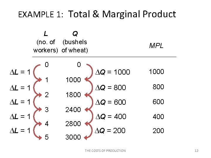
Marginal Product • If Jack hires one more worker, his output rises by the marginal product of labor. • The marginal product of any input is the increase in output arising from an additional unit of that input, holding all other inputs constant. • Notation: ∆ (delta) = “change in…” Examples: ∆Q = change in output, ∆L = change in labor • Marginal product of labor (MPL) = THE COSTS OF PRODUCTION ∆Q ∆L 11

EXAMPLE 1: Total & Marginal Product L Q (no. of (bushels workers) of wheat) ∆L = 1 ∆L = 1 0 0 1 1000 2 1800 3 2400 4 2800 5 3000 MPL ∆Q = 1000 ∆Q = 800 ∆Q = 600 ∆Q = 400 ∆Q = 200 THE COSTS OF PRODUCTION 12

EXAMPLE 1: MPL = Slope of Prod Function Q (no. of (bushels MPL workers) of wheat) 0 1 2 3 4 5 0 1000 1800 2400 2800 3000 1000 800 600 400 200 3, 000 MPL Quantity of output L equals the slope of the 2, 500 production function. 2, 000 Notice that MPL diminishes 1, 500 as L increases. 1, 000 This explains why 500 production the function gets flatter 0 as L 0 increases. 1 2 3 4 5 No. of workers THE COSTS OF PRODUCTION 13

Why MPL Is Important • Recall one of the Ten Principles: Rational people think at the margin. • When Farmer Jack hires an extra worker, – his costs rise by the wage he pays the worker – his output rises by MPL • Comparing them helps Jack decide whether he would benefit from hiring the worker. THE COSTS OF PRODUCTION 14

Why MPL Diminishes • Farmer Jack’s output rises by a smaller and smaller amount for each additional worker. Why? • As Jack adds workers, the average worker has less land to work with and will be less productive. • In general, MPL diminishes as L rises whether the fixed input is land or capital (equipment, machines, etc. ). • Diminishing marginal product: the marginal product of an input declines as the quantity of the input increases (other things equal) THE COSTS OF PRODUCTION 15

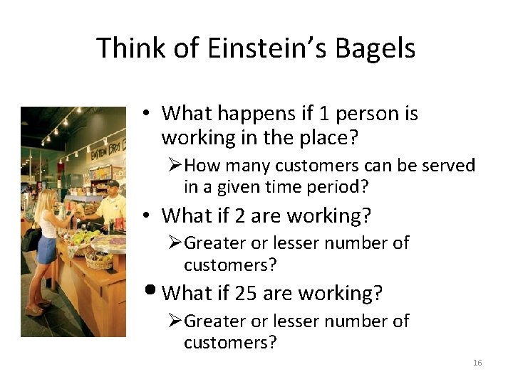
Think of Einstein’s Bagels • What happens if 1 person is working in the place? ØHow many customers can be served in a given time period? • What if 2 are working? ØGreater or lesser number of customers? • What if 25 are working? ØGreater or lesser number of customers? 16

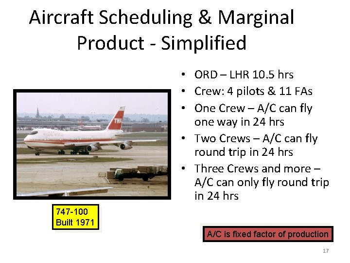
Aircraft Scheduling & Marginal Product - Simplified • ORD – LHR 10. 5 hrs • Crew: 4 pilots & 11 FAs • One Crew – A/C can fly one way in 24 hrs • Two Crews – A/C can fly round trip in 24 hrs • Three Crews and more – A/C can only fly round trip in 24 hrs 747 -100 Built 1971 A/C is fixed factor of production 17

Chapter 13 Outline Explicit vs Implicit Costs Economic vs. Accounting Profit Economies & Diseconomies of Scale Production Function & Marginal Product Costs: Short Run vs. Long Run Costs and Relationship to Output THE COSTS OF PRODUCTION 18

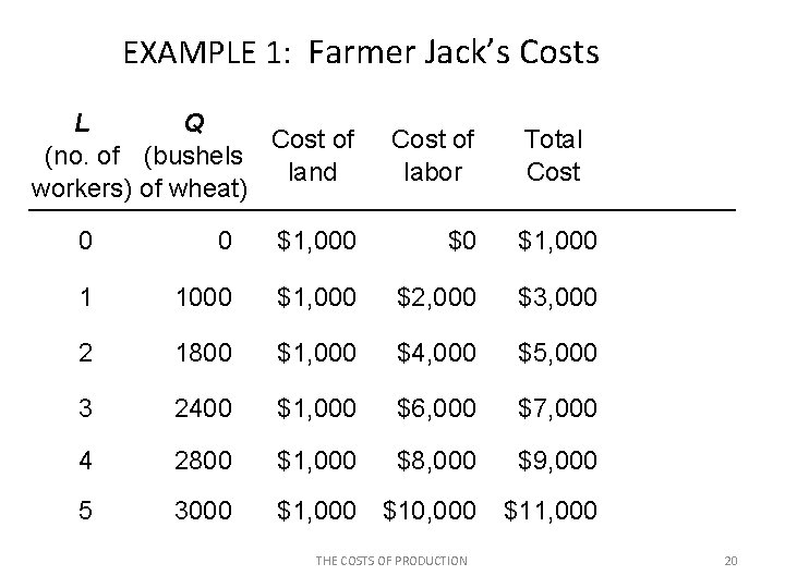
EXAMPLE 1: Farmer Jack’s Costs • Farmer Jack must pay $1000 per month for the land, regardless of how much wheat he grows. • The market wage for a farm worker is $2000 per month. • So Farmer Jack’s costs are related to how much wheat he produces…. THE COSTS OF PRODUCTION 19

EXAMPLE 1: Farmer Jack’s Costs L Q Cost of (no. of (bushels land workers) of wheat) Cost of labor Total Cost 0 0 $1, 000 $0 $1, 000 1 1000 $1, 000 $2, 000 $3, 000 2 1800 $1, 000 $4, 000 $5, 000 3 2400 $1, 000 $6, 000 $7, 000 4 2800 $1, 000 $8, 000 $9, 000 5 3000 $1, 000 $10, 000 $11, 000 THE COSTS OF PRODUCTION 20

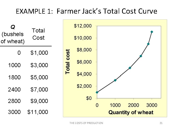
EXAMPLE 1: Farmer Jack’s Total Cost Curve Q (bushels of wheat) Total Cost 0 $1, 000 1000 $3, 000 1800 $5, 000 2400 $7, 000 2800 $9, 000 3000 $11, 000 THE COSTS OF PRODUCTION 21

Marginal Cost • Marginal Cost (MC) is the increase in Total Cost from producing one more unit: ∆TC MC = ∆Q THE COSTS OF PRODUCTION 22

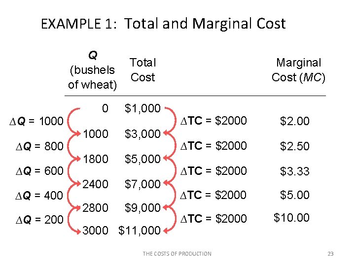
EXAMPLE 1: Total and Marginal Cost Q (bushels of wheat) ∆Q = 1000 ∆Q = 800 ∆Q = 600 ∆Q = 400 ∆Q = 200 Total Cost 0 $1, 000 1000 $3, 000 1800 $5, 000 2400 $7, 000 2800 $9, 000 3000 $11, 000 Marginal Cost (MC) ∆TC = $2000 $2. 00 ∆TC = $2000 $2. 50 ∆TC = $2000 $3. 33 ∆TC = $2000 $5. 00 ∆TC = $2000 $10. 00 THE COSTS OF PRODUCTION 23

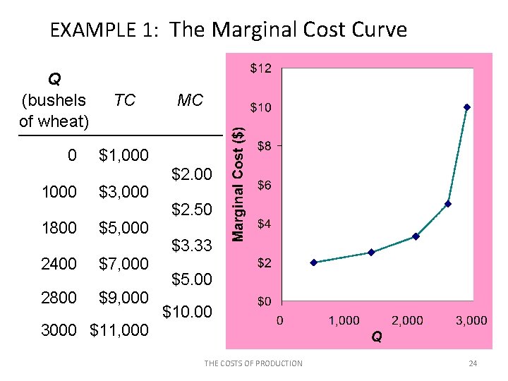
EXAMPLE 1: The Marginal Cost Curve Q (bushels of wheat) 0 TC MC MC usually rises as Q rises, as in this example. $1, 000 1000 $3, 000 1800 $5, 000 2400 $7, 000 2800 $9, 000 3000 $11, 000 $2. 50 $3. 33 $5. 00 $10. 00 THE COSTS OF PRODUCTION 24

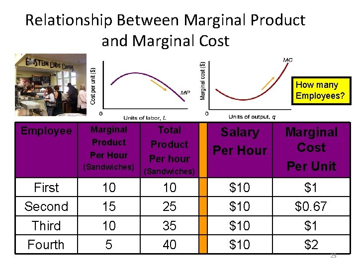
Relationship Between Marginal Product and Marginal Cost How many Employees? Employee Marginal Product Per Hour (Sandwiches) First Second Third Fourth 10 15 10 5 Total Product Per hour Salary Per Hour Marginal Cost Per Unit $10 $10 $1 $0. 67 $1 $2 (Sandwiches) 10 25 35 40 25

Why MC Is Important • Farmer Jack is rational and wants to maximize his profit. To increase profit, should he produce more or less wheat? • To find the answer, Farmer Jack needs to “think at the margin. ” • If the cost of additional wheat (MC) is less than the revenue he would get from selling it, then Jack’s profits rise if he produces more. THE COSTS OF PRODUCTION 26

Fixed and Variable Costs • Fixed costs (FC) do not vary with the quantity of output produced. – For Farmer Jack, FC = $1000 for his land – Other examples: cost of equipment, loan payments, rent • Variable costs (VC) vary with the quantity produced. – For Farmer Jack, VC = wages he pays workers – Other example: cost of materials • Total cost (TC) = FC + VC THE COSTS OF PRODUCTION 27

EXAMPLE 2 • Our second example is more general, applies to any type of firm producing any good with any types of inputs. THE COSTS OF PRODUCTION 28

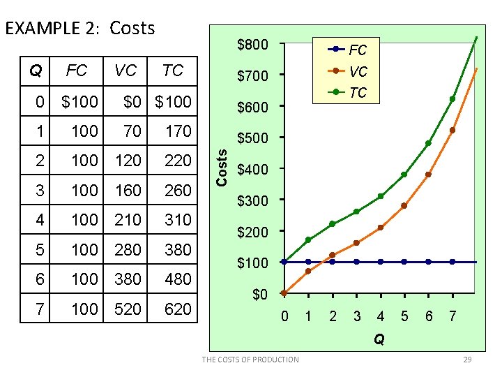
EXAMPLE 2: Costs Q FC VC TC $800 FC $700 VC $0 $100 $600 1 100 70 170 $500 2 100 120 220 3 100 160 260 4 100 210 310 5 100 280 380 6 100 380 480 7 100 520 620 Costs 0 $100 TC $400 $300 $200 $100 $0 0 1 2 3 4 5 6 7 Q THE COSTS OF PRODUCTION 29

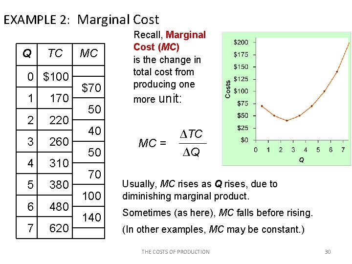
EXAMPLE 2: Marginal Cost Q TC 0 $100 1 170 2 220 3 260 4 310 5 380 6 480 7 620 MC $70 50 40 50 70 100 140 Recall, Marginal Cost (MC) is the change in total cost from producing one more unit: MC = ∆TC ∆Q Usually, MC rises as Q rises, due to diminishing marginal product. Sometimes (as here), MC falls before rising. (In other examples, MC may be constant. ) THE COSTS OF PRODUCTION 30

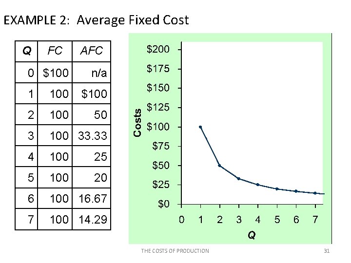
EXAMPLE 2: Average Fixed Cost Q FC 0 $100 AFC n/a 1 100 $100 2 100 50 3 100 33. 33 4 100 25 5 100 20 6 100 16. 67 7 100 14. 29 Average fixed cost (AFC) is fixed cost divided by the quantity of output: AFC = FC/Q Notice that AFC falls as Q rises: The firm is spreading its fixed costs over a larger and larger number of units. THE COSTS OF PRODUCTION 31

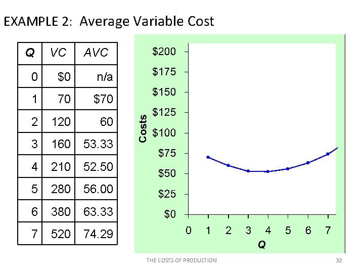
EXAMPLE 2: Average Variable Cost Q VC AVC 0 $0 n/a 1 70 $70 2 120 60 3 160 53. 33 4 210 52. 50 5 280 56. 00 6 380 63. 33 7 520 74. 29 Average variable cost (AVC) is variable cost divided by the quantity of output: AVC = VC/Q As Q rises, AVC may fall initially. In most cases, AVC will eventually rise as output rises. THE COSTS OF PRODUCTION 32

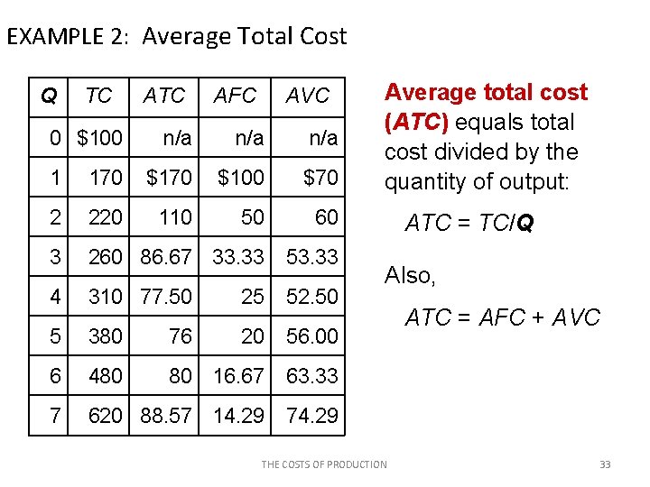
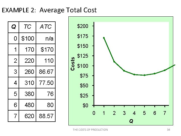
EXAMPLE 2: Average Total Cost Q TC 0 $100 ATC AFC AVC n/a n/a 1 170 $100 $70 2 220 110 50 60 3 260 86. 67 33. 33 53. 33 4 310 77. 50 25 52. 50 5 380 76 20 56. 00 6 480 80 16. 67 63. 33 7 620 88. 57 14. 29 74. 29 Average total cost (ATC) equals total cost divided by the quantity of output: ATC = TC/Q Also, THE COSTS OF PRODUCTION ATC = AFC + AVC 33

EXAMPLE 2: Average Total Cost TC 0 $100 1 170 ATC $200 Usually, as in this example, $175 the ATC curve is U-shaped. n/a $150 $170 110 Costs Q $125 2 220 3 260 86. 67 4 310 77. 50 $50 5 380 76 $25 6 480 80 $0 7 620 88. 57 $100 $75 0 1 2 3 4 5 6 7 Q THE COSTS OF PRODUCTION 34

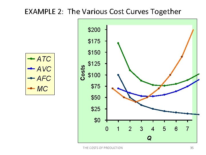
EXAMPLE 2: The Various Cost Curves Together $200 $175 Costs ATC AVC AFC MC $150 $125 $100 $75 $50 $25 $0 0 1 2 3 4 5 6 7 Q THE COSTS OF PRODUCTION 35

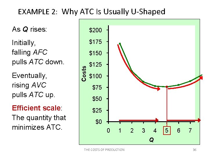
EXAMPLE 2: Why ATC Is Usually U-Shaped As Q rises: $200 Initially, falling AFC pulls ATC down. $175 Efficient scale: The quantity that minimizes ATC. Costs Eventually, rising AVC pulls ATC up. $150 $125 $100 $75 $50 $25 $0 0 1 2 3 4 5 6 7 Q THE COSTS OF PRODUCTION 36

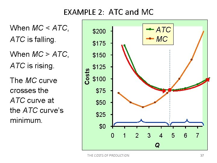
EXAMPLE 2: ATC and MC When MC < ATC, ATC is falling. The MC curve crosses the ATC curve at the ATC curve’s minimum. $175 $150 Costs When MC > ATC, ATC is rising. ATC MC $200 $125 $100 $75 $50 $25 $0 0 1 2 3 4 5 6 7 Q THE COSTS OF PRODUCTION 37

Chapter 13 Outline Explicit vs Implicit Costs Economic vs. Accounting Profit Economies & Diseconomies of Scale Production Function & Marginal Product Costs: Short Run vs. Long Run Costs and Relationship to Output THE COSTS OF PRODUCTION 38

Short-Run Versus Long-Run • The short run is a period of time for which two conditions hold: 1. The firm is operating under a fixed scale (or fixed factor) of production, and 2. Firms can neither enter nor exit the industry. But can shut down 39

Short-Run Versus Long-Run • The long run is a period of time for which there are no fixed factors of production. Firms can increase or decrease scale of operation, and new firms can enter and existing firms can exit the industry. 40

Costs in the Short Run & Long Run • Short run: Some inputs are fixed (e. g. , factories, land). The costs of these inputs are FC. • Long run: All inputs are variable (e. g. , firms can build more factories, or sell existing ones). • In the long run, ATC at any Q is cost per unit using the most efficient mix of inputs for that Q (e. g. , the factory size with the lowest ATC). THE COSTS OF PRODUCTION 41

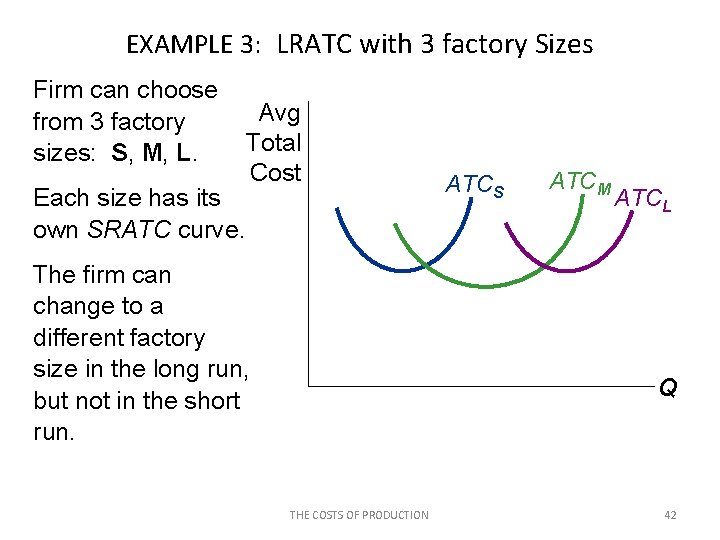
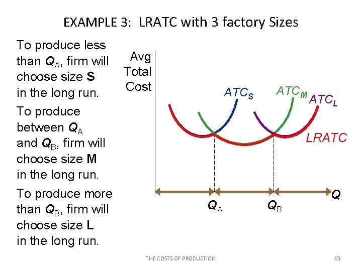
EXAMPLE 3: LRATC with 3 factory Sizes Firm can choose from 3 factory sizes: S, M, L. Each size has its own SRATC curve. Avg Total Cost The firm can change to a different factory size in the long run, but not in the short run. ATCS ATCM ATCL Q THE COSTS OF PRODUCTION 42

EXAMPLE 3: LRATC with 3 factory Sizes To produce less than QA, firm will choose size S in the long run. To produce between QA and QB, firm will choose size M in the long run. To produce more than QB, firm will choose size L in the long run. Avg Total Cost ATCS ATCM ATCL LRATC QA THE COSTS OF PRODUCTION QB Q 43

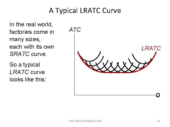
A Typical LRATC Curve In the real world, factories come in many sizes, each with its own SRATC curve. ATC LRATC So a typical LRATC curve looks like this: Q THE COSTS OF PRODUCTION 44

Chapter 13 Outline Explicit vs Implicit Costs Economic vs. Accounting Profit Economies & Diseconomies of Scale Production Function & Marginal Product Costs: Short Run vs. Long Run Costs and Relationship to Output THE COSTS OF PRODUCTION 45

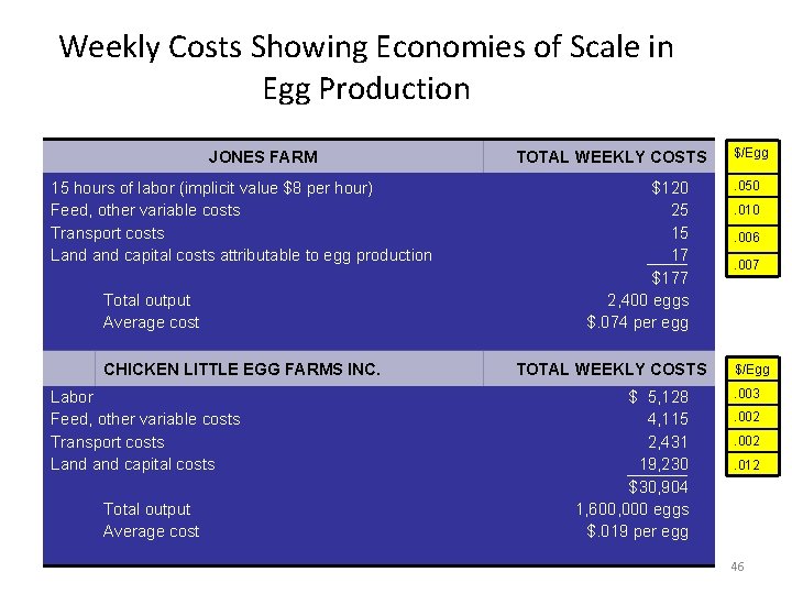
Weekly Costs Showing Economies of Scale in Egg Production JONES FARM 15 hours of labor (implicit value $8 per hour) Feed, other variable costs Transport costs Land capital costs attributable to egg production Total output Average cost CHICKEN LITTLE EGG FARMS INC. Labor Feed, other variable costs Transport costs Land capital costs Total output Average cost TOTAL WEEKLY COSTS $120 25 15 17 $177 2, 400 eggs $. 074 per egg TOTAL WEEKLY COSTS $ 5, 128 4, 115 2, 431 19, 230 $30, 904 1, 600, 000 eggs $. 019 per egg $/Egg. 050. 010. 006. 007 $/Egg. 003. 002. 012 46

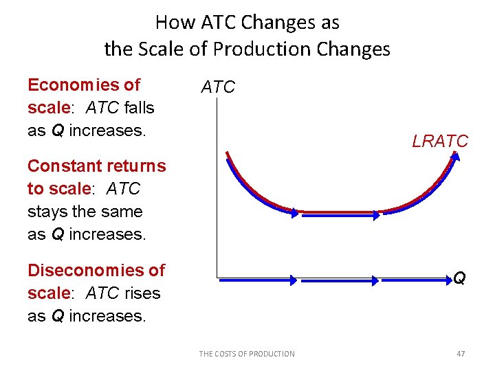
How ATC Changes as the Scale of Production Changes Economies of scale: ATC falls as Q increases. ATC LRATC Constant returns to scale: ATC stays the same as Q increases. Diseconomies of scale: ATC rises as Q increases. Q THE COSTS OF PRODUCTION 47

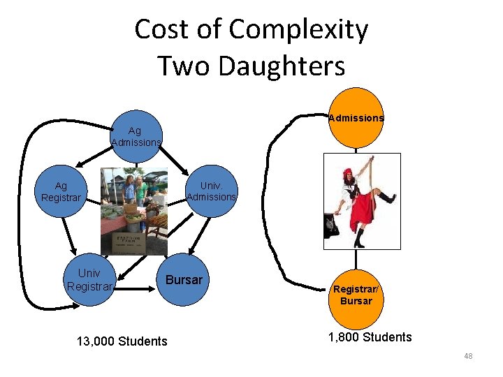
Cost of Complexity Two Daughters Admissions Ag Admissions Univ. Admissions Ag Registrar Student Univ Registrar Bursar 13, 000 Students Registrar/ Bursar 1, 800 Students 48

How ATC Changes as the Scale of Production Changes • Economies of scale occur when increasing production allows greater specialization: workers more efficient when focusing on a narrow task. – More common when Q is low. • Diseconomies of scale are due to coordination problems in large organizations. E. g. , management becomes stretched, can’t control costs. – More common when Q is high. THE COSTS OF PRODUCTION 49

Test Bank Questions THE COSTS OF PRODUCTION 50

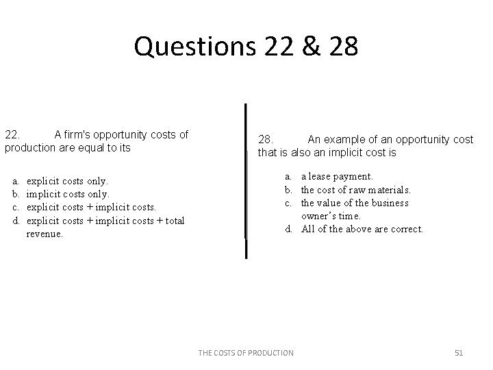
Questions 22 & 28 22. A firm's opportunity costs of production are equal to its a. b. c. d. explicit costs only. implicit costs only. explicit costs + implicit costs + total revenue. 28. An example of an opportunity cost that is also an implicit cost is a. a lease payment. b. the cost of raw materials. c. the value of the business owner’s time. d. All of the above are correct. THE COSTS OF PRODUCTION 51

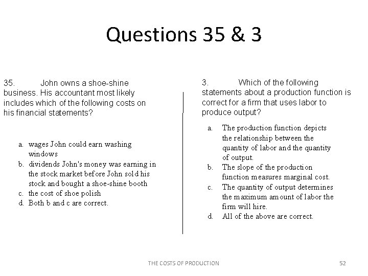
Questions 35 & 3 3. Which of the following statements about a production function is correct for a firm that uses labor to produce output? 35. John owns a shoe-shine business. His accountant most likely includes which of the following costs on his financial statements? a. a. wages John could earn washing windows b. dividends John's money was earning in the stock market before John sold his stock and bought a shoe-shine booth c. the cost of shoe polish d. Both b and c are correct. b. c. d. THE COSTS OF PRODUCTION The production function depicts the relationship between the quantity of labor and the quantity of output. The slope of the production function measures marginal cost. The quantity of output determines the maximum amount of labor the firm will hire. All of the above are correct. 52

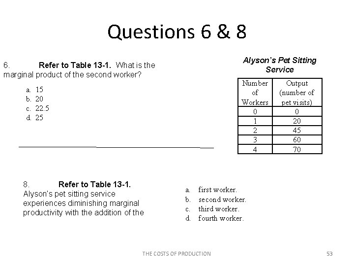
Questions 6 & 8 Alyson’s Pet Sitting Service 6. Refer to Table 13 -1. What is the marginal product of the second worker? a. b. c. d. Number of Workers 0 1 2 3 4 15 20 22. 5 25 8. Refer to Table 13 -1. Alyson’s pet sitting service experiences diminishing marginal productivity with the addition of the a. b. c. d. Output (number of pet visits) 0 20 45 60 70 first worker. second worker. third worker. fourth worker. THE COSTS OF PRODUCTION 53

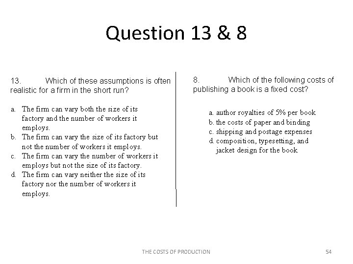
Question 13 & 8 13. Which of these assumptions is often realistic for a firm in the short run? a. The firm can vary both the size of its factory and the number of workers it employs. b. The firm can vary the size of its factory but not the number of workers it employs. c. The firm can vary the number of workers it employs but not the size of its factory. d. The firm can vary neither the size of its factory nor the number of workers it employs. 8. Which of the following costs of publishing a book is a fixed cost? a. author royalties of 5% per book b. the costs of paper and binding c. shipping and postage expenses d. composition, typesetting, and jacket design for the book THE COSTS OF PRODUCTION 54

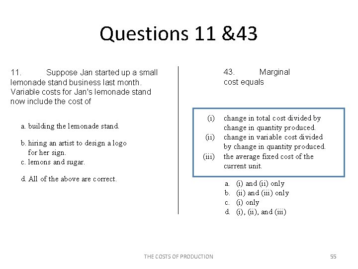
Questions 11 &43 43. Marginal cost equals 11. Suppose Jan started up a small lemonade stand business last month. Variable costs for Jan's lemonade stand now include the cost of a. building the lemonade stand. b. hiring an artist to design a logo for her sign. c. lemons and sugar. (i) (iii) d. All of the above are correct. change in total cost divided by change in quantity produced. change in variable cost divided by change in quantity produced. the average fixed cost of the current unit. a. b. c. d. THE COSTS OF PRODUCTION (i) and (ii) only (ii) and (iii) only (i), (ii), and (iii) 55

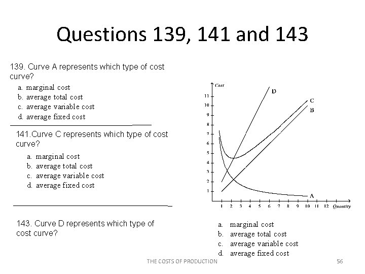
Questions 139, 141 and 143 139. Curve A represents which type of cost curve? a. marginal cost b. average total cost c. average variable cost d. average fixed cost 141. Curve C represents which type of cost curve? a. marginal cost b. average total cost c. average variable cost d. average fixed cost 143. Curve D represents which type of cost curve? THE COSTS OF PRODUCTION a. b. c. d. marginal cost average total cost average variable cost average fixed cost 56

Questions 3 & 19 3. When a factory is operating in the short run, a. it cannot alter variable costs. b. total cost and variable cost are usually the same. c. average fixed cost rises as output increases. d. it cannot adjust the quantity of fixed inputs. 19. Economies of scale arise when a. an economy is self-sufficient in production. b. individuals in a society are selfsufficient. c. fixed costs are large relative to variable costs. d. workers are able to specialize in a particular task. THE COSTS OF PRODUCTION 57

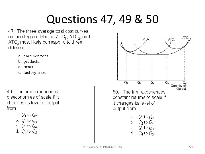
Questions 47, 49 & 50 47. The three average total cost curves on the diagram labeled ATC 1, ATC 2, and ATC 3 most likely correspond to three different a. b. c. d. time horizons. products. firms. factory sizes. 49. The firm experiences diseconomies of scale if it changes its level of output from a. Q 1 to Q 2. b. Q 2 to Q 3. c. Q 3 to Q 4. d. Q 4 to Q 5. 50. The firm experiences constant returns to scale if it changes its level of output from a. b. c. d. THE COSTS OF PRODUCTION Q 1 to Q 2 to Q 4. Q 1 to Q 3. Q 4 to Q 5. 58