The Completely Randomized Design Random samples of size

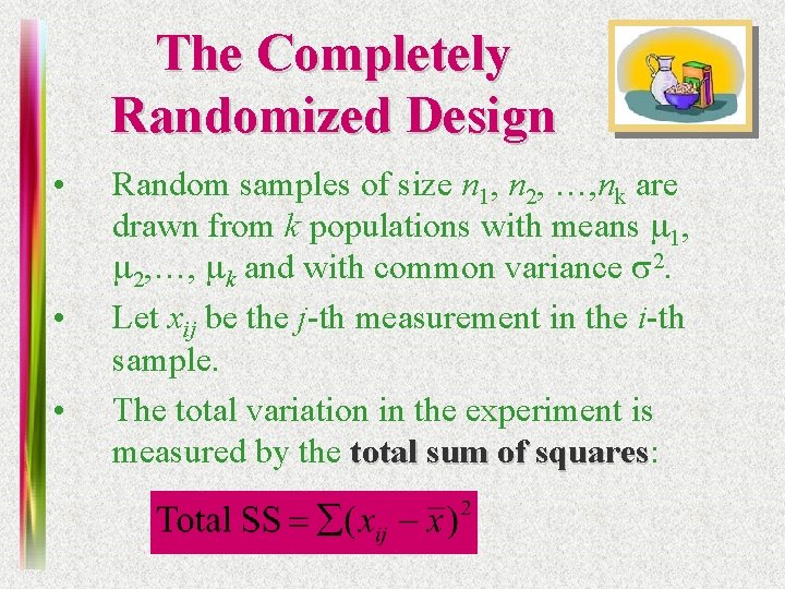
The Completely Randomized Design • • • Random samples of size n 1, n 2, …, nk are drawn from k populations with means m 1, m 2, …, mk and with common variance s 2. Let xij be the j-th measurement in the i-th sample. The total variation in the experiment is measured by the total sum of squares: squares

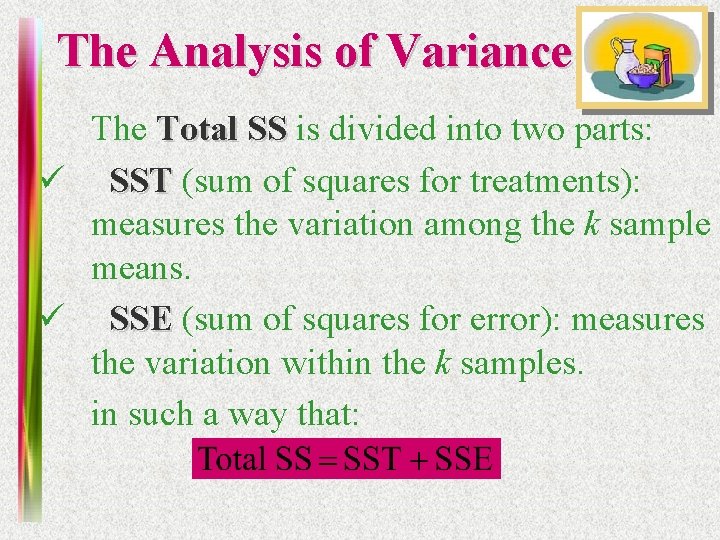
The Analysis of Variance The Total SS is divided into two parts: ü SST (sum of squares for treatments): measures the variation among the k sample means. ü SSE (sum of squares for error): measures the variation within the k samples. in such a way that:

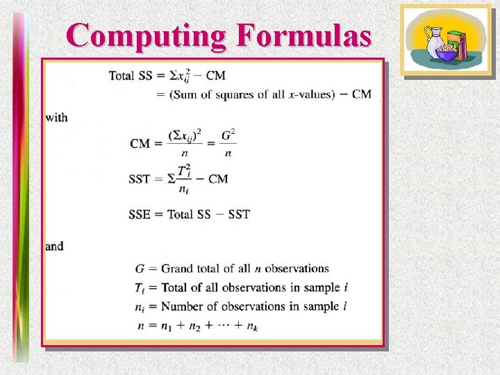
Computing Formulas

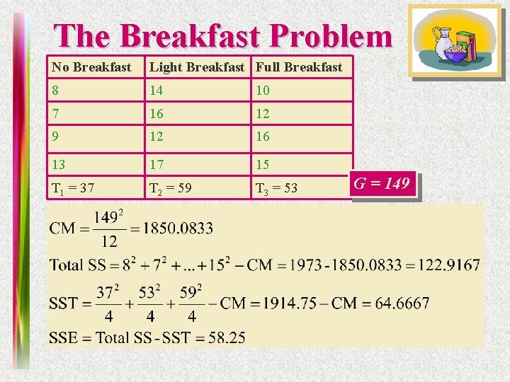
The Breakfast Problem No Breakfast Light Breakfast Full Breakfast 8 14 10 7 16 12 9 12 16 13 17 15 T 1 = 37 T 2 = 59 T 3 = 53 G = 149

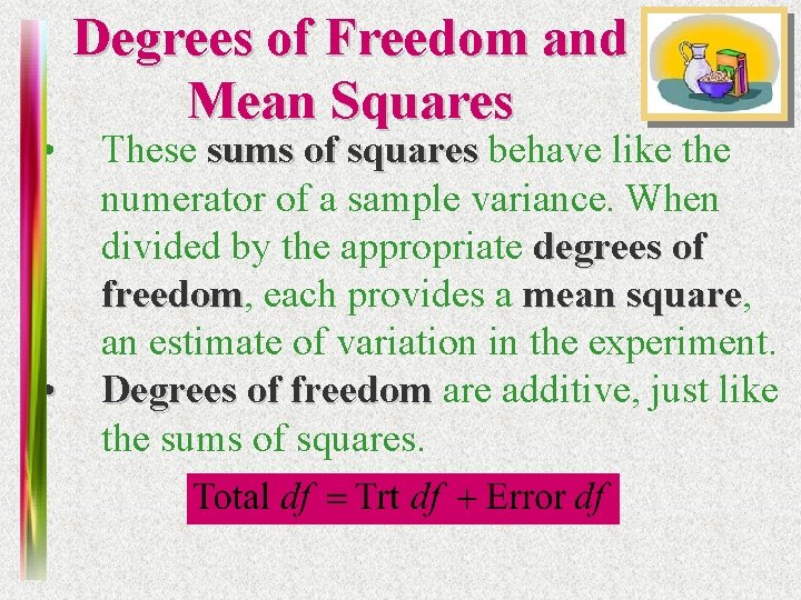
• • Degrees of Freedom and Mean Squares These sums of squares behave like the numerator of a sample variance. When divided by the appropriate degrees of freedom, freedom each provides a mean square, square an estimate of variation in the experiment. Degrees of freedom are additive, just like the sums of squares.

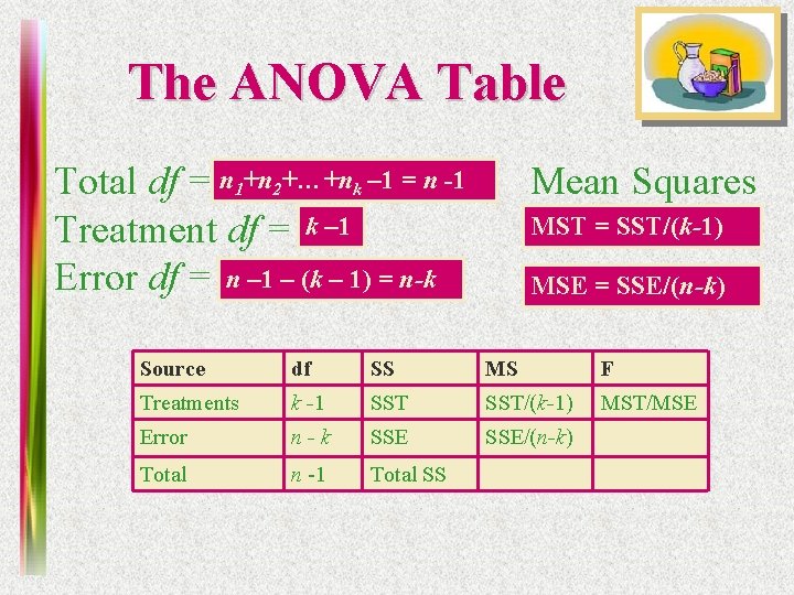
The ANOVA Table Total df = n 1+n 2+…+nk – 1 = n -1 Treatment df = k – 1 Error df = n – 1 – (k – 1) = n-k Mean Squares MST = SST/(k-1) MSE = SSE/(n-k) Source df SS MS F Treatments k -1 SST/(k-1) MST/MSE Error n-k SSE/(n-k) Total n -1 Total SS

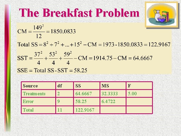
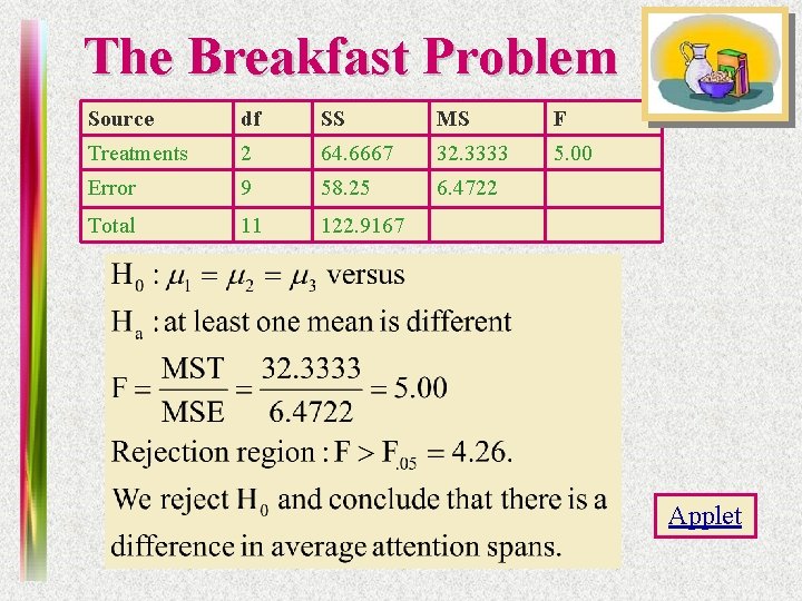
The Breakfast Problem Source df SS MS F Treatments 2 64. 6667 32. 3333 5. 00 Error 9 58. 25 6. 4722 Total 11 122. 9167

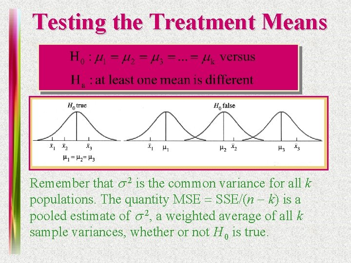
Testing the Treatment Means Remember that s 2 is the common variance for all k populations. The quantity MSE = SSE/(n - k) is a pooled estimate of s 2, a weighted average of all k sample variances, whether or not H 0 is true.

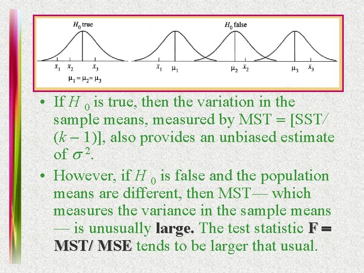
• If H 0 is true, then the variation in the sample means, measured by MST = [SST/ (k - 1)], also provides an unbiased estimate of s 2. • However, if H 0 is false and the population means are different, then MST— which measures the variance in the sample means — is unusually large. The test statistic F = MST/ MSE tends to be larger that usual.

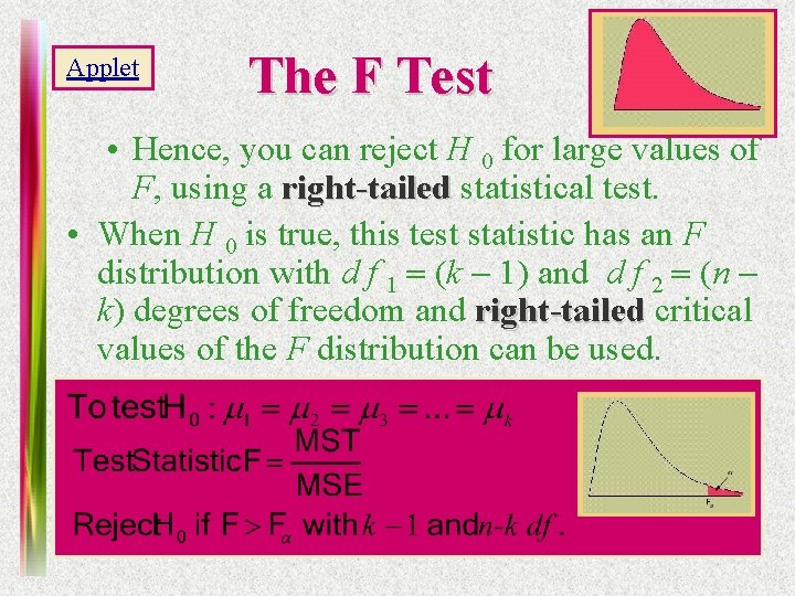
Applet The F Test • Hence, you can reject H 0 for large values of F, using a right-tailed statistical test. • When H 0 is true, this test statistic has an F distribution with d f 1 = (k - 1) and d f 2 = (n k) degrees of freedom and right-tailed critical values of the F distribution can be used.

The Breakfast Problem Source df SS MS F Treatments 2 64. 6667 32. 3333 5. 00 Error 9 58. 25 6. 4722 Total 11 122. 9167 Applet

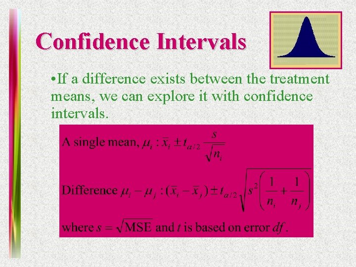
Confidence Intervals • If a difference exists between the treatment means, we can explore it with confidence intervals.

Tukey’s Method for Paired Comparisons • Designed to test all pairs of population means simultaneously, with an overall error rate of a. • Based on the studentized range, range the difference between the largest and smallest of the k sample means. • Assume that the sample sizes are equal and calculate a “ruler” that measures the distance required between any pair of means to declare a significant difference.

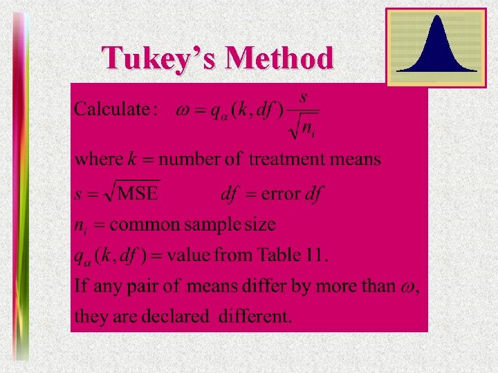
Tukey’s Method

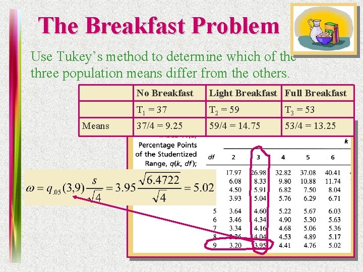
The Breakfast Problem Use Tukey’s method to determine which of the three population means differ from the others. Means No Breakfast Light Breakfast Full Breakfast T 1 = 37 T 2 = 59 T 3 = 53 37/4 = 9. 25 59/4 = 14. 75 53/4 = 13. 25

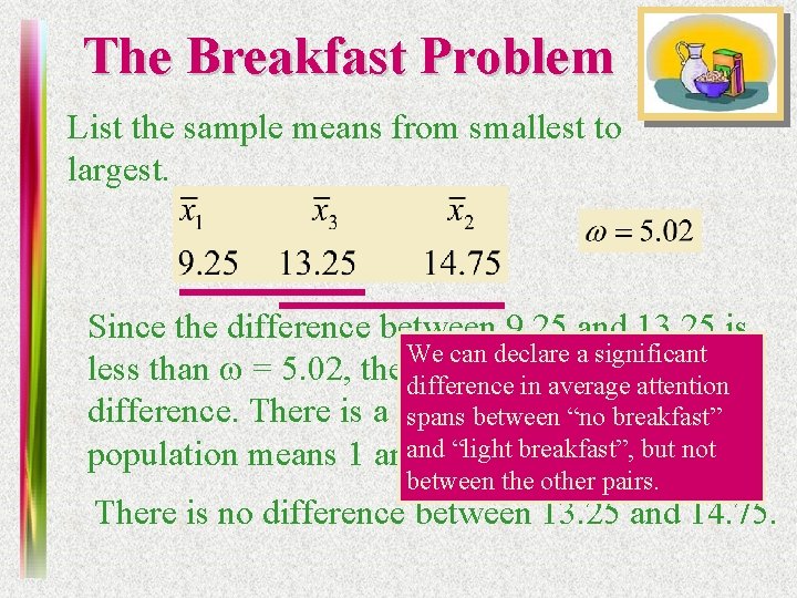
The Breakfast Problem List the sample means from smallest to largest. Since the difference between 9. 25 and 13. 25 is We can declare a significant less than w = 5. 02, there is no significant difference in average attention difference. There is a difference spans between “no breakfast” and 2“light breakfast”, but not population means 1 and however. between the other pairs. There is no difference between 13. 25 and 14. 75.