The CMS Experiment at LHC The CMS Experiment

The CMS Experiment at LHC

The CMS Experiment at LHC A che serve LHC? Macchina di “scoperta” ● A che serve CMS? Esperimento di “scoperta” • Come si fa a scoprire “qualcosa”? ● Tre modi fondamentalmente: A) Si cerca “qualcosa” dove ci si aspetta di trovarlo; (es. quark Top, bosone di Higgs) B) Si cercano eventuali “qualcosa” alla “cieca” (es. supersimmetrie, ricerce di esclusione, etc. ) C) Si cerca un “segnale” di tipo noto anche se non ci sono indicazioni che ci debba essere.

The CMS Experiment at LHC

The CMS Experiment at LHC

Modalità A) di scoperta → La teoria prevede un fenomeno che dovrebbe essere visto effettuando una misura sperimentale. → Esistono misure più o meno indirette che limitano l'intervallo di esistenza del fenomeno (es. massa quark top). Misure dirette (CDF) Mtop = 172 Ge. V Misure indirette

Modalità B) di scoperta → La teoria prevede un fenomeno che dovrebbe essere visto effettuando una misura sperimentale. → Non esistono limiti stringenti sull'intervallo di esistenza del fenomeno (es. ricerca supersimmetrie). Zona permessa

Modalità C) di scoperta → Si cerca un fenomeno che non é previsto dalla teoria. → Es. Ricerca di risonanze nella distribuzione della massa invariante di due jet. La motivazione è che se un pogetto sconosciuto viene prodotto, deve decadere in oggetti noti, prima o poi, che possono quindi essere rivelati.

Cosa guardare? Evento H → ZZ → 4 Che cosa si misura? Z decade rapidissimamente. . . Nessun sensore può vederlo direttamente. Ogni Z decade in altre particelle. Alcune sono sufficientemente stabili perché possano raggiungere dei rivelatori. Es. .

Cosa guardare? Evento H → ZZ → 4 Che cosa si misura? Z decade rapidissimamente. . . Nessun sensore può vederlo direttamente. Ogni Z decade in altre particelle. Alcune sono sufficientemente stabili perché possano raggiungere dei rivelatori. Es. .

Evento H → ZZ → 4 “Golden Channel” Occorre trovare 4 m soddisfacenti alla condizione pt > 25 Ge. V

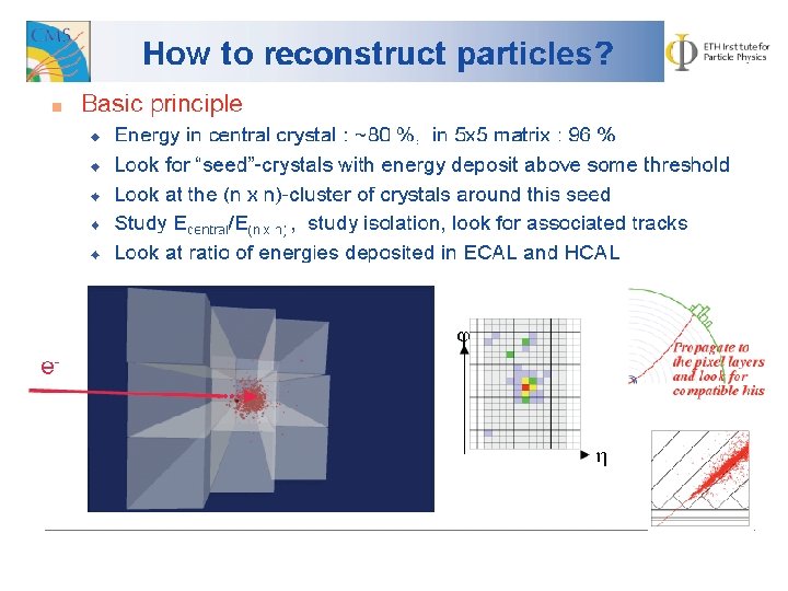
Ricerca di “oggetti fisici” Quindi occorre essere in grado di rivelare una serie di “oggetti fisici” che sono i prodotti finali decadimenti che si vogliono studiare. → → → muoni elettroni tau fotoni jet → energia mancante (un caso diverso → neutrini e altro)

Ricerca di “oggetti fisici”

Chi fa cosa. . .

Rivelazione di particelle cariche Serve un magnete che pieghi la traiettoria delle particelle nel piano perpendicolare alla direzione del campo magnetico (piano r-f)

The Tracker System Concept: Rely on “few” measurement layers, each able to provide robust (clean) and precise coordinate determination 2 to 3 Silicon Pixel, and 10 to 14 Silicon Strip Measurement Layers Radius ~ 110 cm, Length ~ 270 cm ~1. 7 R-phi (Z-phi) only measurement layers 6 layers TOB R-phi (Z-phi) & Stereo measurement layers ~2. 4 4 layers TIB Goal: p. T ~ 1 -2% * p. T Pixel Vertex 3 disks TID 9 disks TEC

The concept in reality:

Quali sensori? Silicon detectors Come funzionano i rivelatori a silicio? Microstrips Rivelatore polarizzato inversamente per avere un volume completamente svuotato da portatori maggioritari. 300 – 500 m

Module components production & assembly The numbers 6, 136 Thin + 18, 192 Thick sensors 440 m 2 of silicon wafers 210 m 2 of silicon sensors Large scale industrial sensor production 9, 648, 128 strips channels 75, 376 APV chips Reliable, High Yield Industrial IC process Hybrids Pitch adapters Frames 6, 136 Thin sensor modules (1 sensor / module) 9, 096 Thick sensor modules (2 sensors / module) Automated module assembly 25, 000 wire bonds State of the art bonding machines

Shells, Rods and Petals

The Concept Silicon Pixel vertex detector

Putting it in perspective Tracker read-out dominates CMS data volume CMS Silicon Strip Tracker has no 0 suppression: CMM noise subtraction (Pixels have local 0 suppression => intrinsic noise immunity crucial) Analogue information from all 107 strips/event read-out at 100 KHz event rate Use analogue optical link: developed for Tracker now used throughout CMS After digitization and 0 suppression in the FED, Tracker data volume ~ / event => Drives requirements of DAQ Opto-hybrid Distributed Patch Panel Receiver Module Inline Patch Panel 12 96 FED Detector Hybrid 1 TOB TEC TIB TID CMS Cavern Counting Room

Quali sensori? Silicon detectors

The Concept Silicon Pixel vertex detector The region below 20 cm is instrumented with Silicon Pixel Vertex systems (First layer at R ~ 4 cm) 4 107 pixels The Pixel area is driven by FE chip The shape is optimized for resolution CMS pixel ~ 100 m * 150 m Shaping time ~ 25 ns With this cell size, and exploiting the large Lorentz angle We obtain IPtrans. resolution ~ 20 m for tracks with Pt ~ 10 Ge. V cm 30 With this cell size occupancy is ~ 10 -4 m 93 c This makes Pixel seeding the fastest Starting point for track reconstruction Despite the extremely high track density

The Silicon Tracker Concept: expected performance The CMS Tracker provides ~ 1% Pt resolution over ~ 0. 9 units of , and 2% Pt resolution up to ~ 1. 75, beyond which the lever arm is reduced With material Without / with material Even at 100 Ge. V muons are significantly affected by multiple scattering: a finer pitch, and higher channel count Would therefore yield only diminishing returns in improving the Pt resolution

The Silicon Tracker Concept expected performance: For 10 Ge. V Pt tracks, (d 0) < 30 for < 1. 5; degrading to ~ 40 for = 2. 4 10 Ge. V For 10 Ge. V Pt tracks, (Z 0) < 50 for < 1. 5; degrading to ~ 150 for = 2. 4 Dominated by Pixel geometry and multiple scattering

Resistance to Radiation Damage

The Silicon Sensors The reverse biased p-on-n diode Bulk depletes from P+ implants, “front-side“ to N+ implant, “back-side ” Electron-hole pairs generated in the depleted region drift to the N+ and P+ electrodes respectively and generate a signal ~ to the depleted sensor thickness Electron-hole pairs generated in the (conductive) un-depleted region recombine locally, and generate no signal Even in a partially depleted sensor, the signal on the “front-side” is localized Oxide Al Strips OV P+ implants N Bulk N+ Implants - -+ + - -+ + - + +HV

The Silicon Sensors Radiation damaged reverse biased p-on-n diode Radiation damage eventually results in “type inversion” The initially N bulk undergoes “type inversion” and becomes P The depletion voltage decreases and then increases again with higher fluence The effectively P bulk depletes from N+ implants, “back-side”, to P+ implant, “front-side” Electron-hole pairs generated in the depleted region drift to the N+ and P+ electrodes respectively and generate a signal ~ to the depleted sensor thickness Radiation induced defects trap charge, leading to a loss of signal unless high fields In the partially depleted sensor, the signal on the “front-side” is no longer localized Sensor leakage current increases linearly with fluence (by ~ 3 orders of magnitude) Al Strips P+ implants P bulk N+ Implants - - -+ -+ - ++ OV +HV

The Silicon Sensors The radiation hard P-on-N strip detector Radiation hardness “recipe” P-on-N sensors work after bulk type inversion, Provided they are biased well above depletion At room temperature and above, radiation induced defects diffuse and some eventually form clusters which further increase the sensor depletion voltage “reverse annealing” Defect mobility below ~ 0 C is sufficient low that reverse annealing is effectively frozen out Maintain radiation damaged silicon below ~0 C (constantly) Sensor leakage current depends ~ exponentially on temperature: it doubles for every ~7 C temperature increase Insufficient cooling efficiency will result in an exponential “thermal run-away” of the irradiated sensor Operate sensors below ~ -10 C, to reduce required cooling efficiency & material

The Silicon Sensors The radiation hard P-on-N strip detector Radiation hardness “recipe” P-on-N sensors work after bulk type inversion, Provided they are biased well above depletion Optimize design for high voltage stability, as well as low capacitance Use Al layer as field plate to remove high field at strip edges from Si bulk to Oxide (much higher Vbreak) Strip width/pitch ~ 0. 25: reduce Ctot while maintaining stable high bias voltage operation (avoid strip pitch > 200 m to ensure stable high voltage operation) Surface damage P+ implants “P” Bulk +++ ----++ Surface radiation damage can increase strip capacitance & noise, and degrade high voltage stability +++ ----++ +++++ ----- Use <100> crystal instead of <111> Take care with process: implants, oxides… N+ Implants

The Silicon Sensors The radiation hard P-on-N strip detector Radiation hardness “recipe” P-on-N sensors work after bulk type inversion, Provided they are biased well above depletion Match sensor thickness (& resistivity) to fluence (Vdep) to optimize S/N over the full life-time: Use 320 m thickness for R < 60 cm, Strip ~ 10 cm => S/N ~ 18 (14) Use 500 m thickness for R > 60 cm, Strip ~ 20 cm => S/N ~ 21 (16)

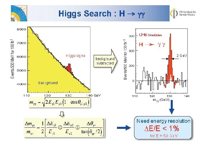
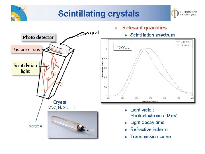
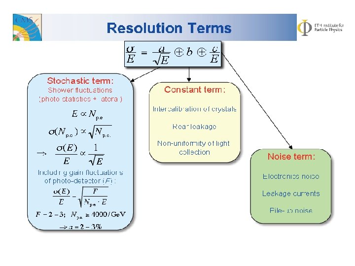
Calorimetria elettromagnetica

Calorimetria elettromagnetica

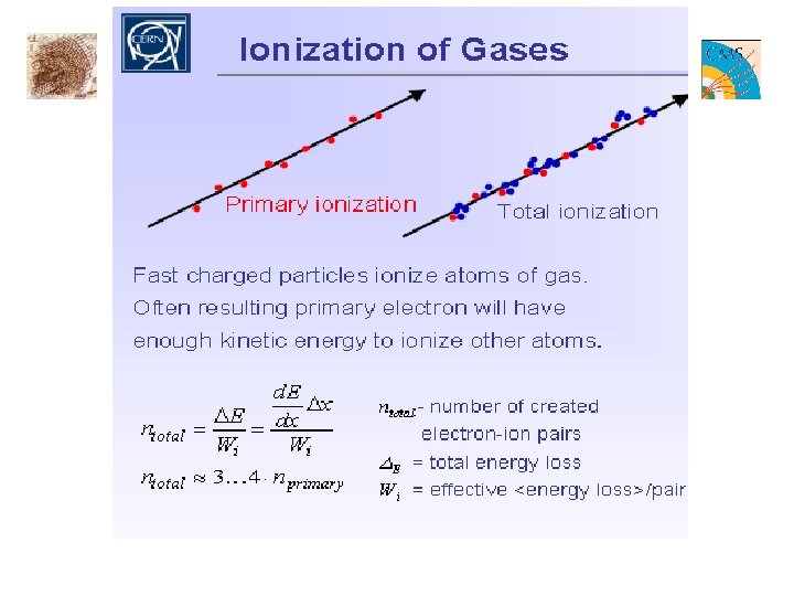
Calorimetria adronica

Calorimetria adronica Sciame adronico

Calorimetria adronica

Calorimetria adronica

Muon Detectors

Muon Detectors

Muon Detectors

Muon Detectors

Muon Detectors

Muon Detectors

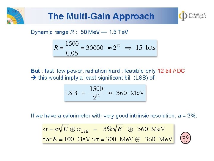
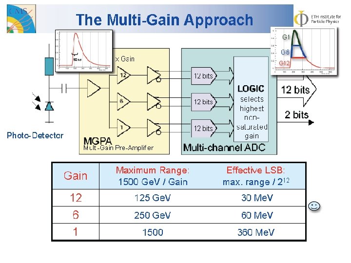
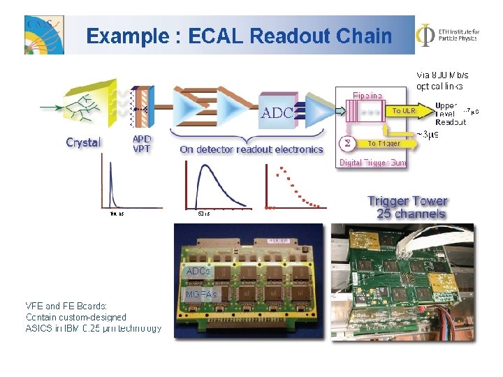
Lettura dei segnali Il problema della rivelazione di segnali comprende la parte della loro lettura , trattamento e trasmissione al sistema di Acquisizione Dati. Problema molto spesso fondamentale!

Catena di Lettura Calorimetro elettromagnetico

Material in the Tracker volume Cables required to bring 16 KA in and out of active volume Cooling required to absorb ~ 40 k. W dissipated in active volume Mechanics to support all this, and ensure accurate & stable sensor placement

Tracker Alignment Mechanical Constraints & Metrology: Sensors on Modules ~ 10 m Modules within Sub-Structures 0. 1~ 0. 5 mm Sub-Structures within Support Tube ~ few mm Laser Alignment System: Aligns Sub-Structures & monitors relative movements at the level of ~ 10 m Expect to ensure ~ few 100 m alignment uncertainties Sufficient for a first efficient pattern recognition

Impact of alignment on Physics Use Z to illustrate ~ 2. 4 Ge. V Ideal detector First Data Taking <1 fb-1 Laser Alignment Mechanical Constraints ≈100 m alignment uncertainties ~ 2. 9 Ge. V Mz Mz ~ 3. 5 Ge. V Mz First Data Taking: 1 fb-1 First results of Alignment with tracks ≈20 m alignment uncertainties

Track reconstruction, ossia come passare dai punti alla traccia → impulso Use Pixel layers for seeding: Lowest occupancy (despite highest track density) Full 3 -dimensional coordinate determination Beam spot constraint

Track Reconstruction Robust pattern recognition The three Pixel layers, with the beam spot constraint, play a crucial role in ensuring a manageable track ambiguity level at the seed generation stage: Requiring 2/3 pixel hits for a seed, and with relatively loose beam spot constraints, 1/15 (1/35) pixel seeds is reconstructed as a track at low (high) luminosity respectively (This ratio is substantially higher for seeds with 3 pixel hits, but imposing This requirement would lead to significant inefficiencies)

Track Reconstruction Track parameter resolution vs. # of hits Good track parameter resolution already with 4 or more hits

Event selection Questi decadono secondo i vari canali: es. H → 4 m Di questi solo alcuni sono rivelati: Efficienza

Event selection

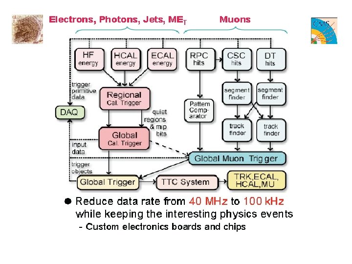
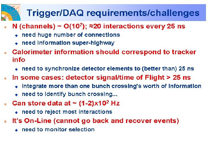
Perchè così poco tempo? pp collision @ 14 Te. V @ 1034 cm-2 s-1 every 25 ns

È sufficiente tutto questo? No. . .

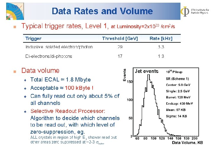
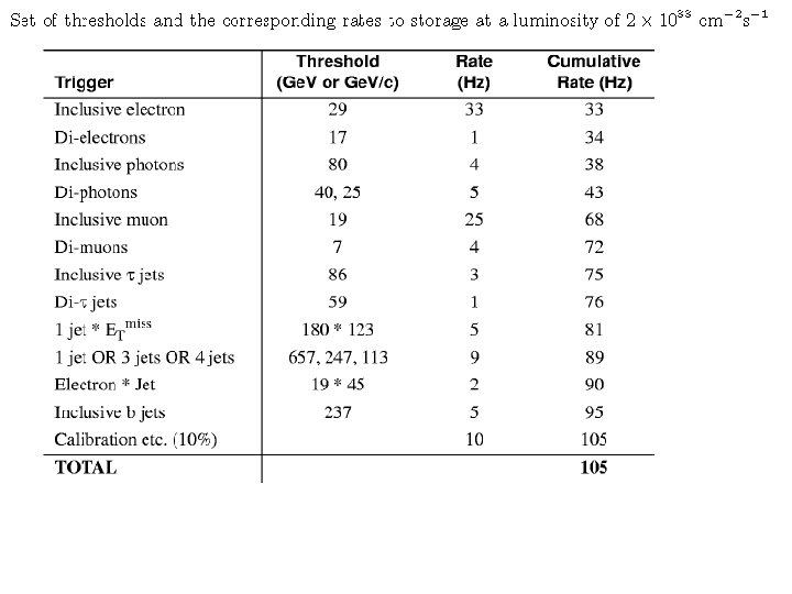
Tabella riassuntiva rate principali triggers

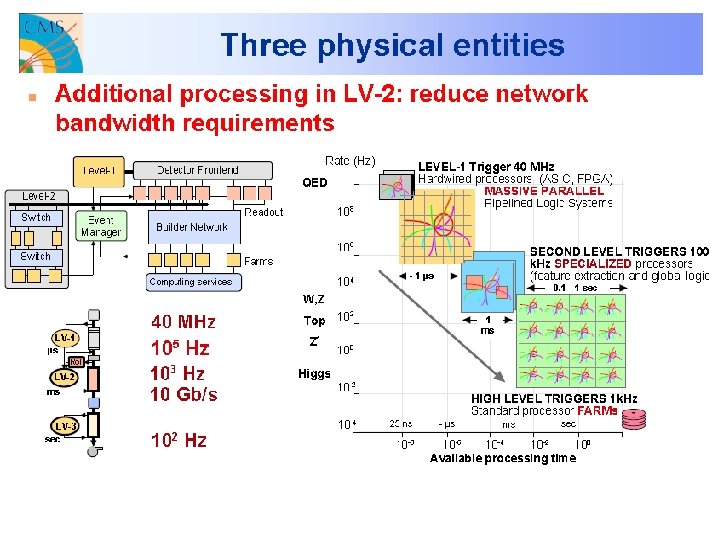
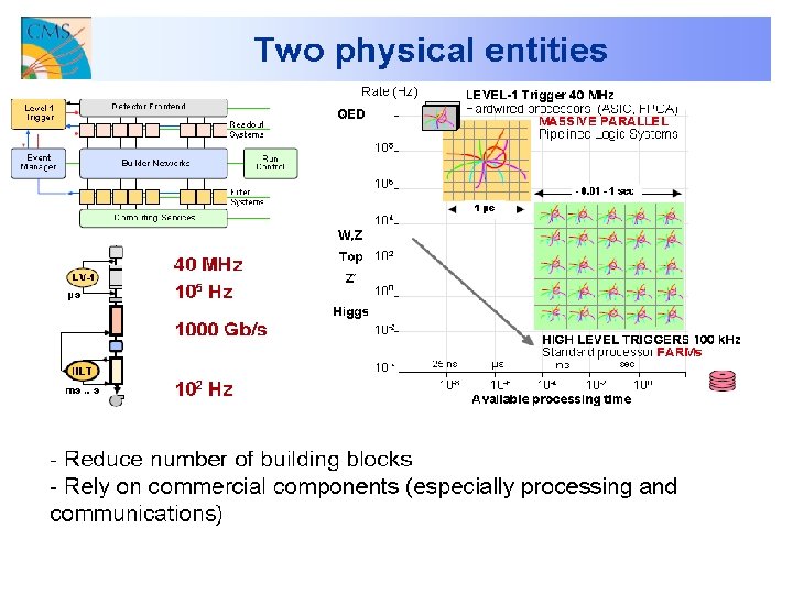
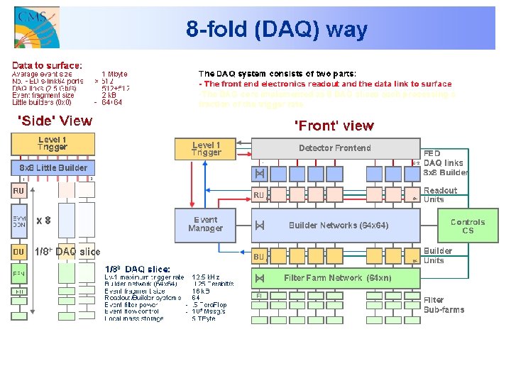
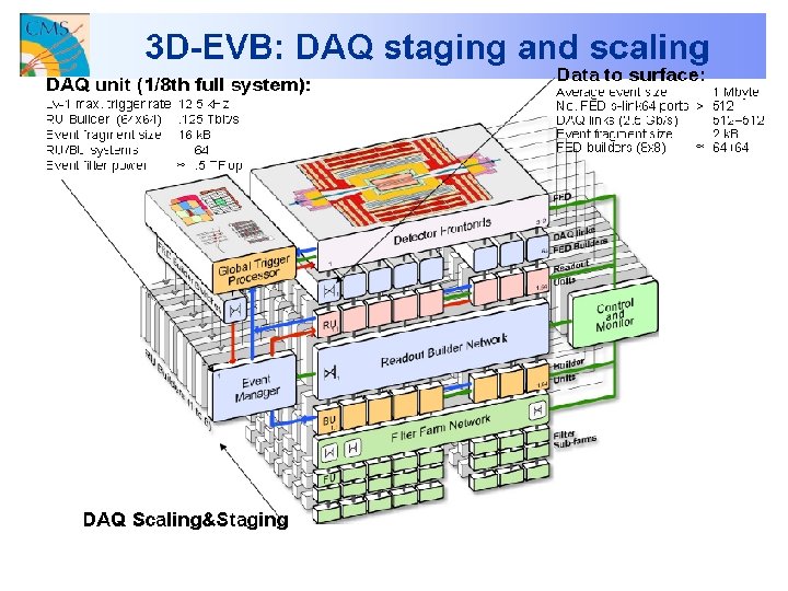
The Tracker at HLT CMS L 1 Trigger and HLT farm filter Lvl-1 = “crude” granularity and Pt resolution: Rate dominated by miss-measured jets & leptons HLT task: reduce rate by ~ 1000 Exploit much better Granularity and Pt resolution to correctly tag and retain only interesting physics events On average ~300 ms available for HLT Decision on any given event (Normalized to a 1 GHz Pentium) 40 MHZ 50 KHz 100 Hz 4 DAQ slices in 2007 => 50 KHZ into HLT, 100 Hz out

The Tracker at HLT for example t lepton tagging Regional Tracking: Look only in Jet-track matching cone Conditional Tracking: Stop track as soon as If Pt<1 Ge. V with high C. L. Reject event if no “leading track found” (jet is not charged) Regional Tracking: Look only inside Isolation cone Conditional Tracking: Stop track as soon as If Pt<1 Ge. V with high C. L. Reject event as soon as additional track found (jet is not isolated) Fast enough at low luminosity for full L 1 rate; at high luminosity may need a moderate Calorimeter pre-selection factor to reduce rate

È sufficiente tutto questo? No. . . Per la prevista fase 2 di LHC (LHC High Luminosity - SLHC) si prevede un fattore 10 di luminosità in più.

È sufficiente tutto questo? No. . . Il trigger attuale non funzionerà più:

È sufficiente tutto questo? No. . .

È sufficiente tutto questo? No. . .

È sufficiente tutto questo? No. . .

Idea concettuale: doppio stack.

Track reconstruction and pattern matching The pattern matching compares the event with ALL the candidates tracks stored in a local memory (Pattern Bank). The pattern matching can be very fast for online track reconstruction thanks to the Associative Memory (AM) parallelism [see CDF use-case] The Event The Pattern Bank. . .

Workflow of pattern matching Entro 2 - 3 s

Open basic questions. . .

Event Processing parallelization

Open basic questions. . . Occorre trovare un compromesso tra dimensioni del settore, numero di pattern da controllare, numero di settori, …. . . Oggetto di un programma specifico pluriennale di ricerca.