The Case for Classical Spacetime Ken Wharton Department

The Case for Classical Spacetime Ken Wharton Department of Physics and Astronomy San Jose State University

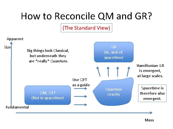
How to Reconcile QM and GR? (The Standard View) Apparent Size GR (In, and of, spacetime) Big things look Classical, but underneath they are *really* Quantum. Use QFT as a guide QM, QFT (Not in spacetime) Hamiltonian GR is emergent, at large scales. Quantum Gravity Spacetime is therefore also emergent. Fundamental Mass

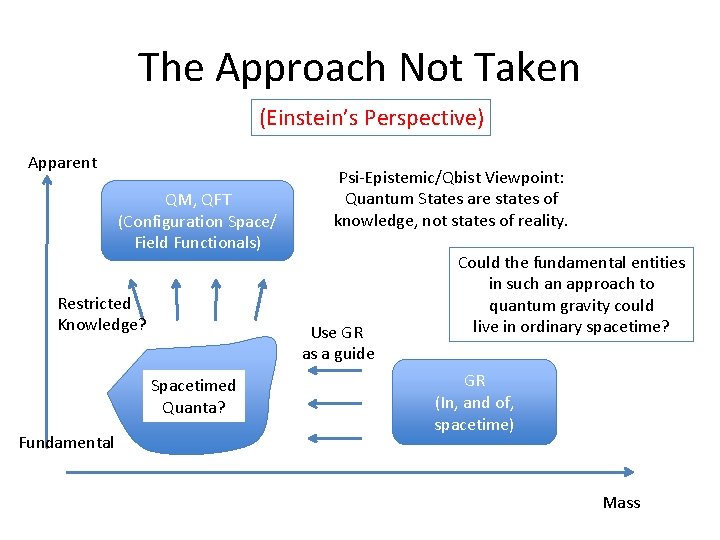
The Approach Not Taken (Einstein’s Perspective) Apparent QM, QFT (Configuration Space/ Field Functionals) Restricted Knowledge? Use GR as a guide Deeper Spacetimed Explanation Quanta? Fundamental Psi-Epistemic/Qbist Viewpoint: Quantum States are states of knowledge, not states of reality. Could the fundamental entities in such an approach to quantum gravity could live in ordinary spacetime? GR (In, and of, spacetime) Mass

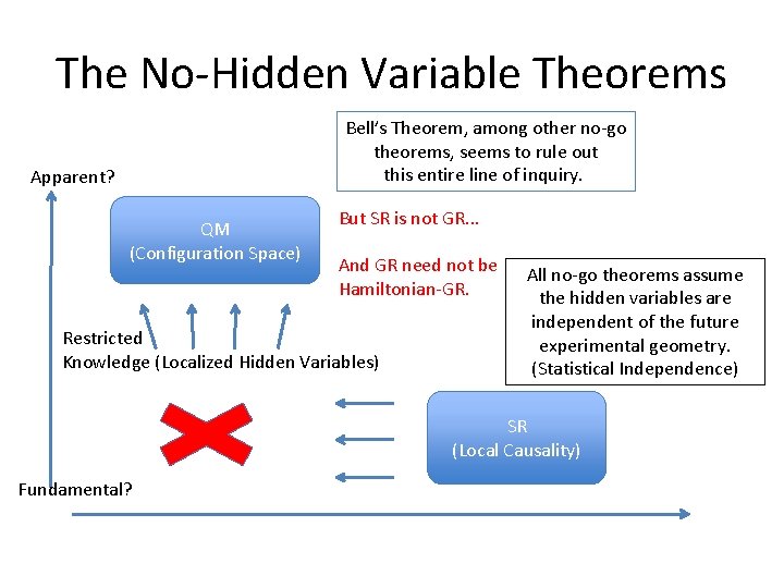
The No-Hidden Variable Theorems Bell’s Theorem, among other no-go theorems, seems to rule out this entire line of inquiry. Apparent? QM (Configuration Space) But SR is not GR. . . And GR need not be Hamiltonian-GR. Restricted Knowledge (Localized Hidden Variables) All no-go theorems assume the hidden variables are independent of the future experimental geometry. (Statistical Independence) SR (Local Causality) Fundamental?

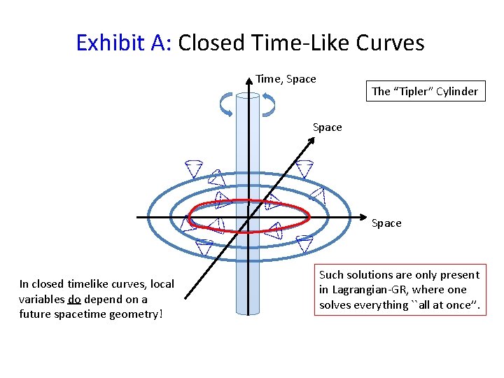
Exhibit A: Closed Time-Like Curves Time, Space The “Tipler” Cylinder Space In closed timelike curves, local variables do depend on a future spacetime geometry! Such solutions are only present in Lagrangian-GR, where one solves everything ``all at once’’.

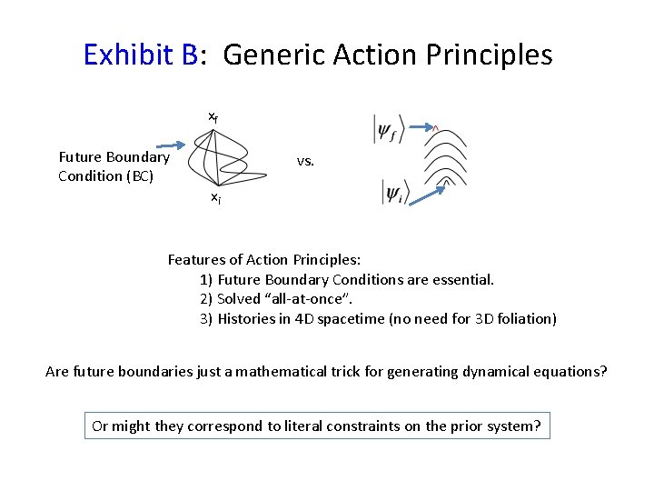
Exhibit B: Generic Action Principles xf Future Boundary Condition (BC) vs. xi Features of Action Principles: 1) Future Boundary Conditions are essential. 2) Solved “all-at-once”. 3) Histories in 4 D spacetime (no need for 3 D foliation) Are future boundaries just a mathematical trick for generating dynamical equations? Or might they correspond to literal constraints on the prior system?

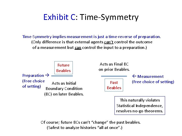
Exhibit C: Time-Symmetry implies measurement is just a time-reverse of preparation. (Only difference is that external agents can’t control the outcome of a measurement but can control the input to a preparation. ) Future Beables Preparation (Free choice Acts as Initial of setting) Boundary Condition Acts as Final BC on prior Beables. Past Beables Measurement (Free choice of setting) (BC) on later Beables. This naturally violates Statistical Independence, resolves no-go theorems. Of course; future BCs can’t “change” the past beables. (Safest to analyze histories “all at once”. )

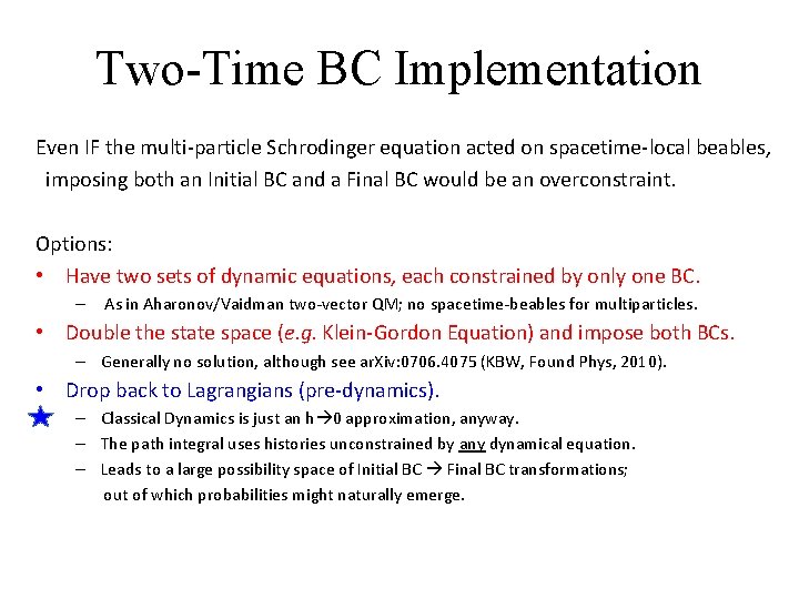
Two-Time BC Implementation Even IF the multi-particle Schrodinger equation acted on spacetime-local beables, imposing both an Initial BC and a Final BC would be an overconstraint. Options: • Have two sets of dynamic equations, each constrained by only one BC. – As in Aharonov/Vaidman two-vector QM; no spacetime-beables for multiparticles. • Double the state space (e. g. Klein-Gordon Equation) and impose both BCs. – Generally no solution, although see ar. Xiv: 0706. 4075 (KBW, Found Phys, 2010). • Drop back to Lagrangians (pre-dynamics). – Classical Dynamics is just an h 0 approximation, anyway. – The path integral uses histories unconstrained by any dynamical equation. – Leads to a large possibility space of Initial BC Final BC transformations; out of which probabilities might naturally emerge.

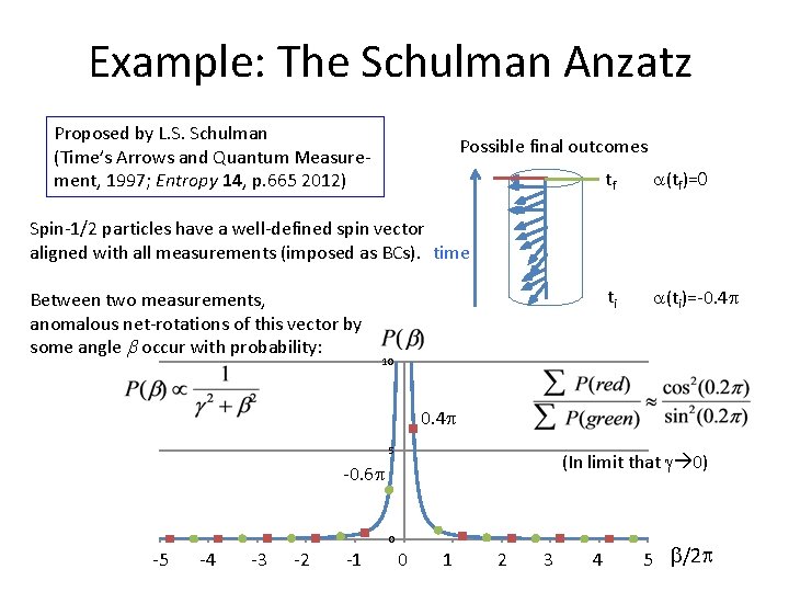
Example: The Schulman Anzatz Proposed by L. S. Schulman (Time’s Arrows and Quantum Measurement, 1997; Entropy 14, p. 665 2012) Possible final outcomes tf a(tf)=0 ti a(ti)=-0. 4 p Spin-1/2 particles have a well-defined spin vector aligned with all measurements (imposed as BCs). time Between two measurements, anomalous net-rotations of this vector by some angle b occur with probability: 10 0. 4 p 5 (In limit that g 0) -0. 6 p 0 -10 -5 -8 -4 -6 -3 -4 -2 -2 -1 00 12 24 36 48 5 b/2 p 10

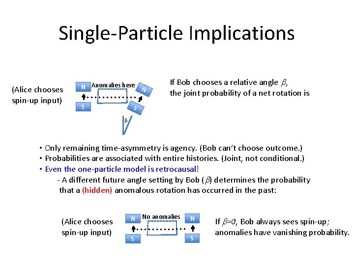
Single-Particle Implications (Alice chooses spin-up input) N Anomalies here N S If Bob chooses a relative angle b, the joint probability of a net rotation is S b • Only remaining time-asymmetry is agency. (Bob can’t choose outcome. ) • Probabilities are associated with entire histories. (Joint, not conditional. ) • Even the one-particle model is retrocausal! - A different future angle setting by Bob (b) determines the probability that a (hidden) anomalous rotation has occurred in the past: (Alice chooses spin-up input) N S No anomalies N S If b=0, Bob always sees spin-up; anomalies have vanishing probability.

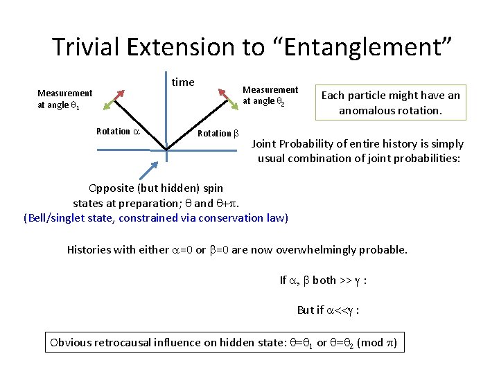
Trivial Extension to “Entanglement” time Measurement at angle q 1 Rotation a Measurement at angle q 2 Rotation b Each particle might have an anomalous rotation. Joint Probability of entire history is simply usual combination of joint probabilities: Opposite (but hidden) spin states at preparation; q and q+p. (Bell/singlet state, constrained via conservation law) Histories with either a=0 or b=0 are now overwhelmingly probable. If a, b both >> g : But if a<<g : Obvious retrocausal influence on hidden state: q=q 1 or q=q 2 (mod p)

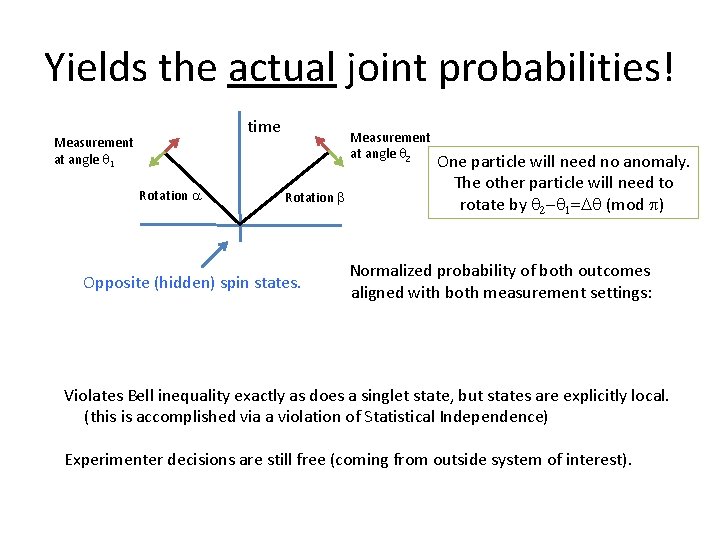
Yields the actual joint probabilities! time Measurement at angle q 1 Rotation a Measurement at angle q 2 Rotation b Opposite (hidden) spin states. One particle will need no anomaly. The other particle will need to rotate by q 2 -q 1=Dq (mod p) Normalized probability of both outcomes aligned with both measurement settings: Violates Bell inequality exactly as does a singlet state, but states are explicitly local. (this is accomplished via a violation of Statistical Independence) Experimenter decisions are still free (coming from outside system of interest).

Further Generalizations • Immediately extends to any maximally-entangled two-qubit state (via rotations). • Partially entangled states require a larger space of hidden variables. – Exactly the right-size HV space is motivated by going to second-order Lagrangians (ar. Xiv: 1411. 4999) – Allows a simple local analog of a Controlled-Not quantum gate (CNOT). • CNOTs and rotations can build any entangled state (in finite dimensional Hilbert Space) – All that is needed is a generalization of Schulman’s Anzatz that reproduces probabilities on such states. Stay Tuned!

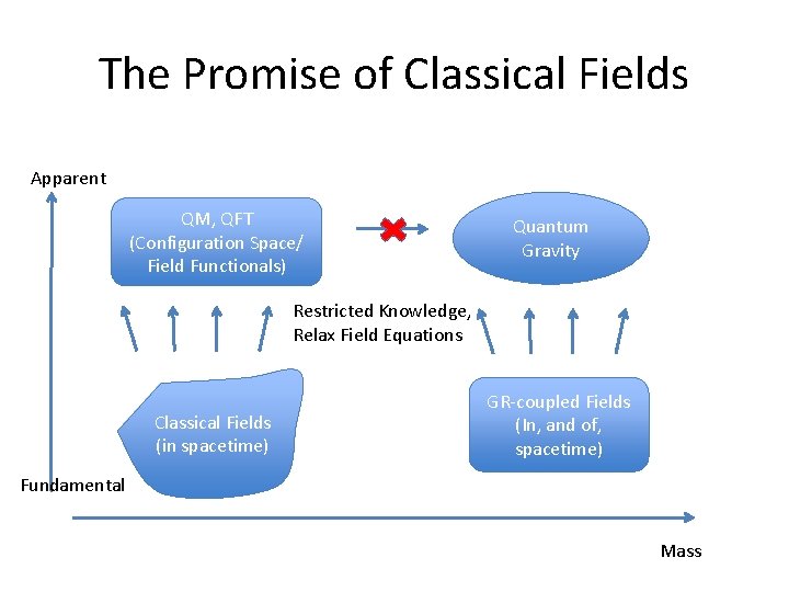
The Promise of Classical Fields Apparent QM, QFT (Configuration Space/ Field Functionals) Quantum Gravity Restricted Knowledge, Relax Field Equations Classical Fields (in spacetime) GR-coupled Fields (In, and of, spacetime) Fundamental Mass

Conclusions • Given future boundaries, spacetime-beables are on the table. – Enormous ontological reduction, for quite a small price. • Configuration space only seems real if one refuses to Bayesianupdate the past (when learning future measurement settings). ar. Xiv: 1403. 2374, KBW Information, v 5 p. 190 (2014). • Lagrangian-style analysis contains all the key ingredients: – All-at-once approach to multi-boundary problems (block universe) – Many possible histories (even when constrained by external geometry) – Proof of principle covers entanglement; about to be fully generalized. • Spacetime might still be emergent, but this would free such approaches from also having to explain quantum phenomena.