The Care and Feeding of Vector Fields Waldo

The Care and Feeding of Vector Fields Waldo Tobler Professor Emeritus of Geography University of California Santa Barbara, CA 93106 -4060 USA http: //www. geog. ucsb. edu/~tobler 1

A Better Title Might Be Creating, using, manipulating, and inverting vector fields. 2

Abstract Objects and observations used in GIS are most often categorical or numerical. An object less frequently represented has both a value and a direction. A common such object, familiar to all, is the slope of a topographic surface. However numerous additional instances give rise to vectors. Well-known operations, such as filtering and interpolation, can be applied to vectors. There also analyses unique to vectors and vector fields. Some of these result in a further generalization, objects that have different magnitudes in all directions, a. k. a. Tensors. 3 Presented to the Association for Geographic Information, London, 27 April 2000

Subjects To Be Covered Partial List Conventional sources of vector fields What can be done with vector fields Increasingly abstract examples Calculating potential fields from tables Resolution and its effects 4

In GIS It Is Common to Refer to Rasters and Vectors. These refer to the format of the data This is NOT what my talk is about! Rather I am looking at the sequence Scalar - Vector - Tensor 5

The Most Frequent Data in a GIS Are Categorical data or Scalar data 6

Examples of Categorical Data Are: Nominal classes such as land use or soil type. These can be given as classes within polygons or by ‘pixels’ in a raster. 7

Single Numbers at Every Place Are Examples of Scalar Data. As for a raster (or TIN) of topographic elevations, or population defined for polygons, etc. 8

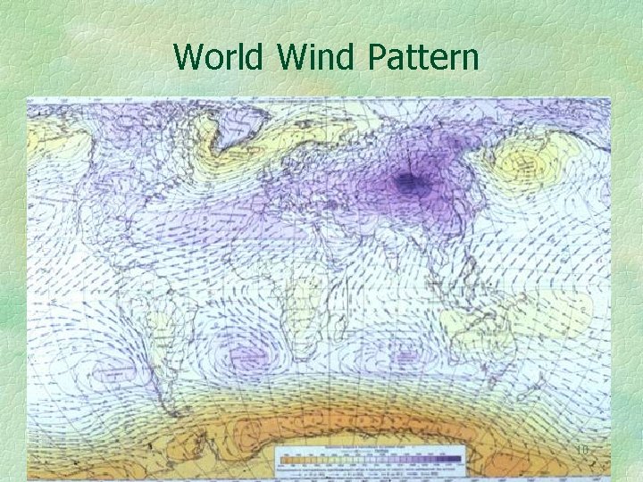
Two Numbers at Every Place Are Examples of Vector Data. Wind speed and direction is a good and well known example of a vector field. 9

World Wind Pattern 10

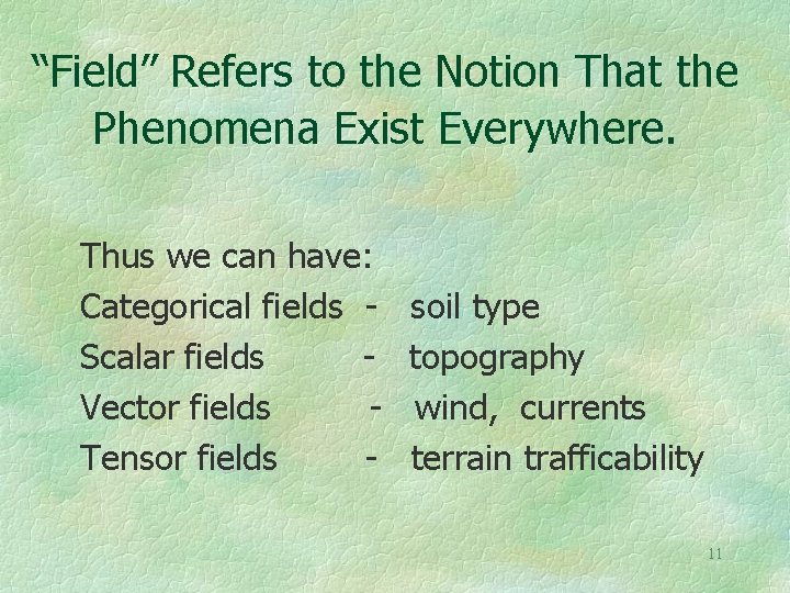
“Field” Refers to the Notion That the Phenomena Exist Everywhere. Thus we can have: Categorical fields Scalar fields Vector fields Tensor fields - soil type topography wind, currents terrain trafficability 11

It Is Not Implied That the Values Have Been Measured Everywhere But that they can conceptually exist everywhere. So a vector field might be sampled, and known, only at isolated locations, or at the vertices of a regular lattice or other tesselation. 12

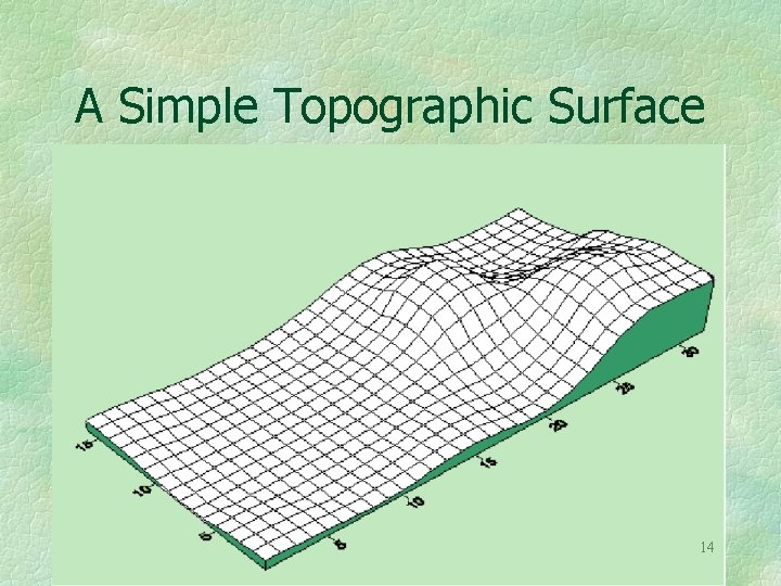
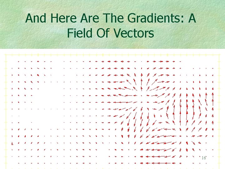
A Familiar Vector Field Can Be Defined For Topography The slope of a topographic surface gives rise to a vector field. For example if we start with 13

A Simple Topographic Surface 14

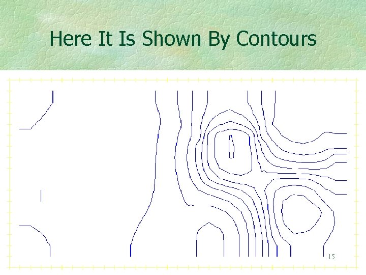
Here It Is Shown By Contours 15

And Here Are The Gradients: A Field Of Vectors 16

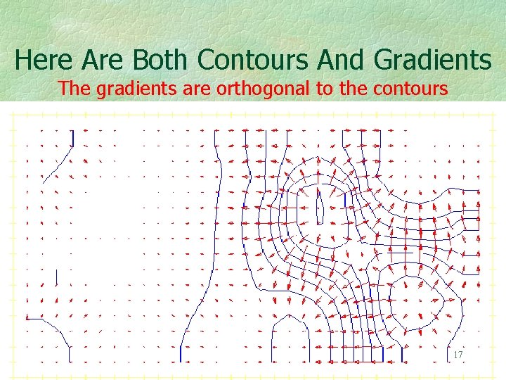
Here Are Both Contours And Gradients The gradients are orthogonal to the contours 17

The Gradient Field Has the First Partial Derivatives of the Topography As Its Components. The derivatives of the vector field give rise to further objects. For example, second derivatives are often used in geophysics to determine the spatial loci of change. They are similar to the Laplacian filters used in remote sensing applications. There may be further uses of these higher derivatives. 18

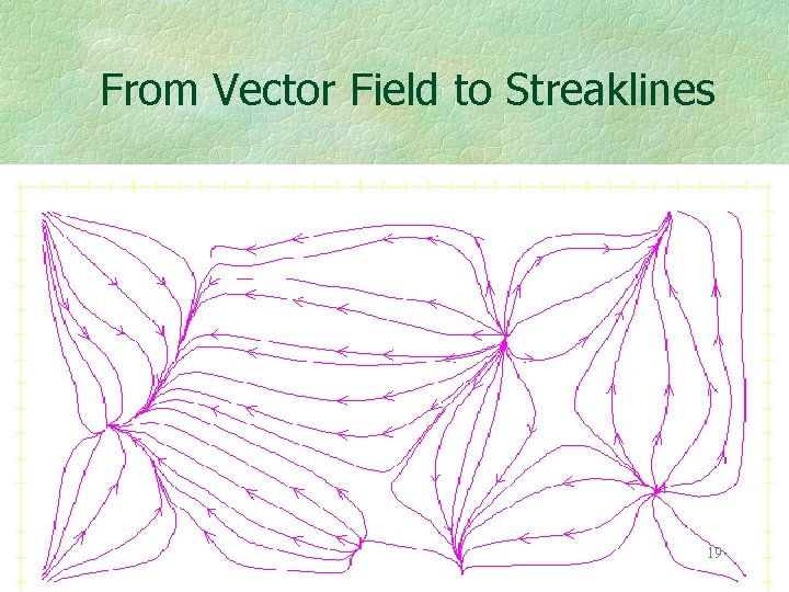
From Vector Field to Streaklines 19

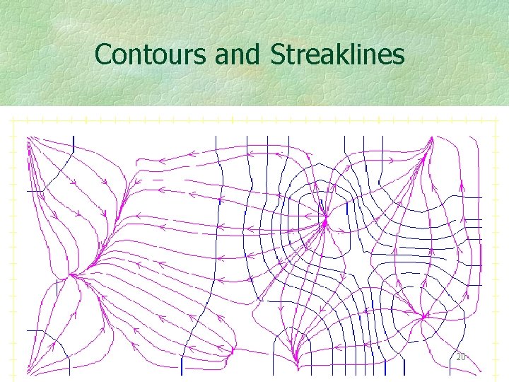
Contours and Streaklines 20

The Streaklines Are Constructed Using the Gradient Vectors As such they are also orthogonal to the contours. Basins may now be delineated Those of you working in physical geography will recognize that producing stream traces is a little more complicated than this. There is a large literature. 21

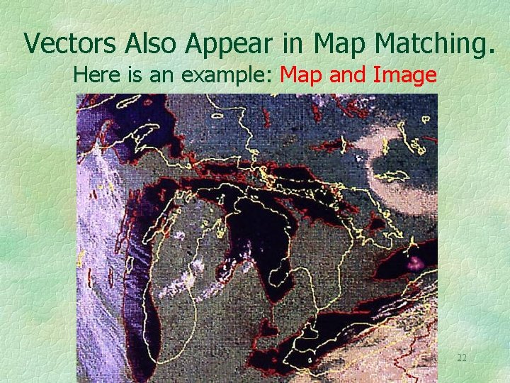
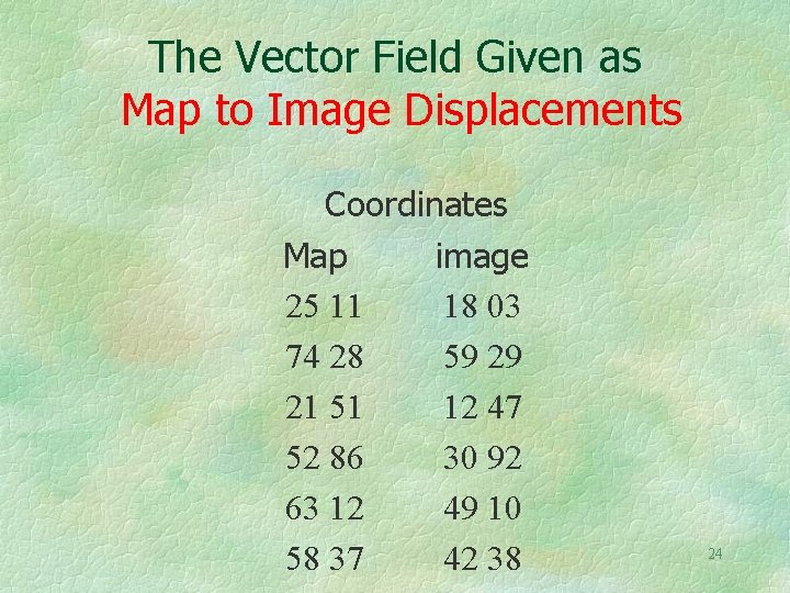
Vectors Also Appear in Map Matching. Here is an example: Map and Image 22

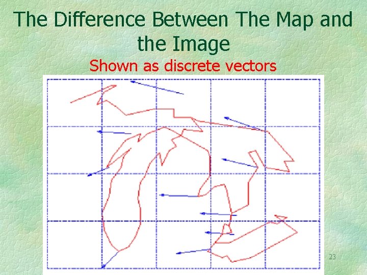
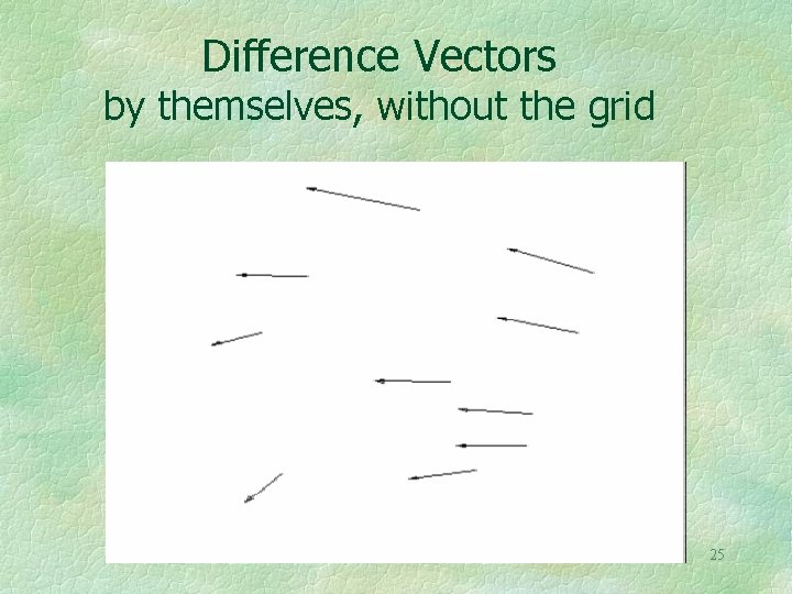
The Difference Between The Map and the Image Shown as discrete vectors 23

The Vector Field Given as Map to Image Displacements Coordinates Map image 25 11 18 03 74 28 59 29 21 51 12 47 52 86 30 92 63 12 49 10 58 37 42 38 24

Difference Vectors by themselves, without the grid 25

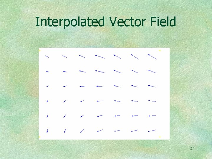
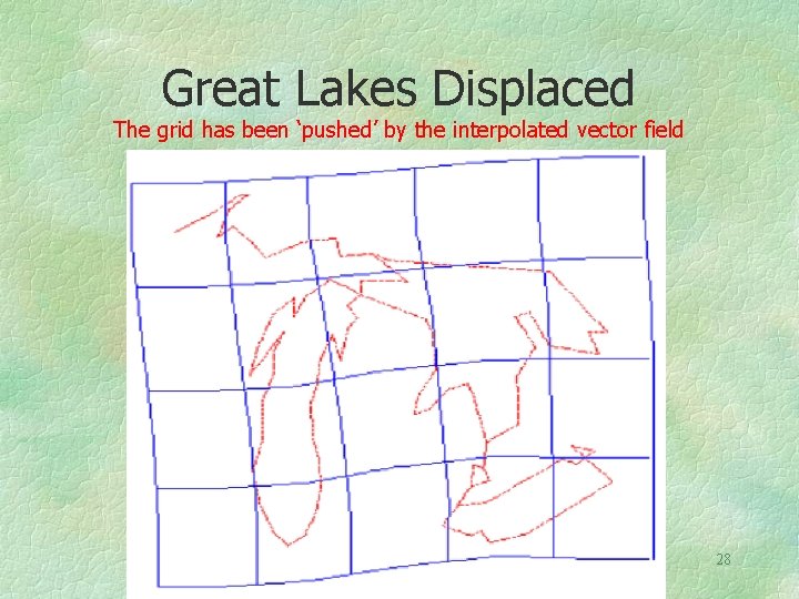
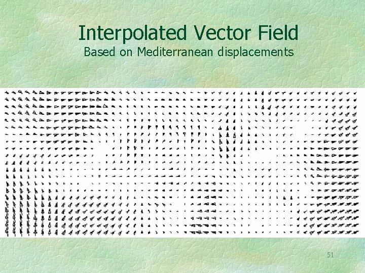
Scattered Vectors Can Be Interpolated to Yield a Vector Field Inverse distance, krieging, splining, or other forms of interpolation may be used. Smoothing or filtering of the scattered vectors or of the vector field can also easily be applied. This is done by applying the operator to the individual vector components. Or treat the vectors as complex numbers with the common properties of numbers. 26

Interpolated Vector Field 27

Great Lakes Displaced The grid has been ‘pushed’ by the interpolated vector field 28

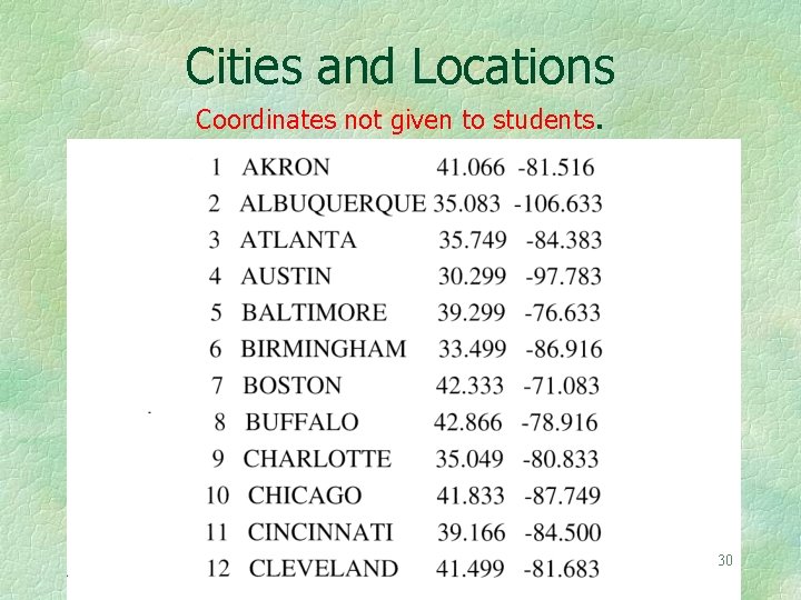
Here Is an Example From the Field Known As ‘Mental Mapping’ A list of the sixty largest US cities, in alphabetical order, is given to students. 29

Cities and Locations Coordinates not given to students. 30

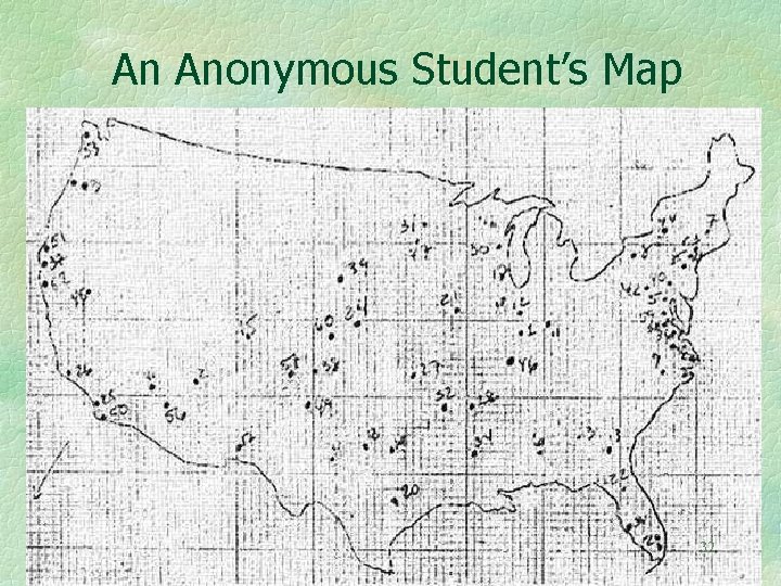
Instructions to the Students Work without any reference materials Use Graph Paper, wide Margin at top. Plot Cities with ID Number on the Graph Paper. USA Outline may be drawn, but is not required. 31

An Anonymous Student’s Map 32

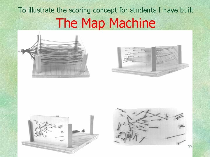
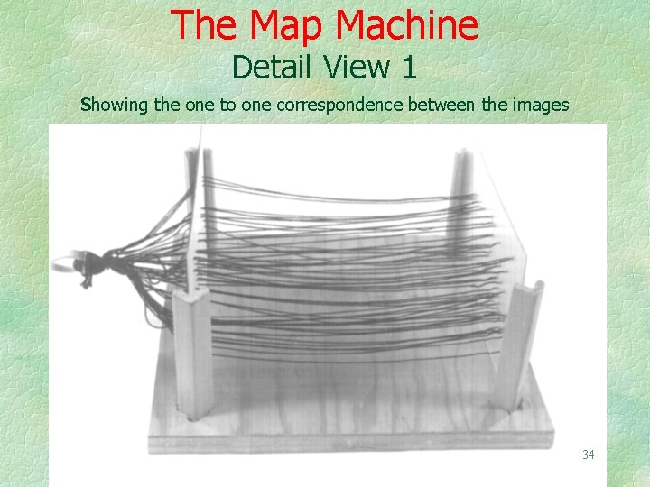
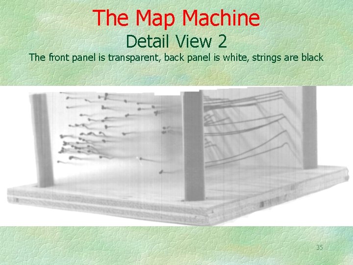
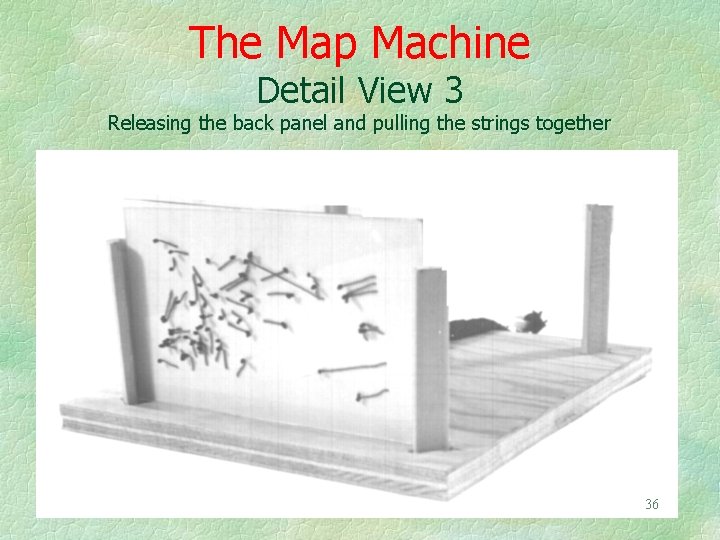
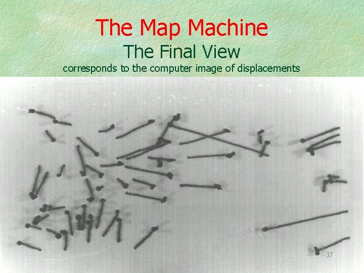
To illustrate the scoring concept for students I have built The Map Machine 33

The Map Machine Detail View 1 showing the one to one correspondence between the images 34

The Map Machine Detail View 2 The front panel is transparent, back panel is white, strings are black 35

The Map Machine Detail View 3 Releasing the back panel and pulling the strings together 36

The Map Machine The Final View corresponds to the computer image of displacements 37

The Student Map Shows Displacement Vectors These vectors could also show change of address coordinates, due to a move. Or they could be home to shopping moves, etc. Thus there are many possible interpretations of this kind of vector displacement 38

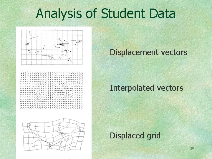
Analysis of Student Data Displacement vectors Interpolated vectors Displaced grid 39

The displaced grid could be used to interpolate a warped map of the United States. Given the severe displacements the map would need to overlap itself 40

With Student Maps In Hand How to score? Compute correlation, R 2, between actual and student estimates? How to do this? Correlation between scores of different students? Factor analyze? Compute vector field variance, etc. , to determine degree of fuzziness? Average vectors over all students? 41

It is often the case that one has several vector fields covering the same geographic area. A simple example would be wind vectors and ocean currents. How can these different fields be compared? 42

Is There a Method of Computing the Correlation Between Vector Fields? The question comes up not only in meteorology and oceanography but also for the comparison of the student’s maps, for comparison of old maps, and in many other situations. There are in fact such correlation methods, and associated with these are regression-like predictors. Statistical significance tests are also available. 43 B. Hanson, et al, 1992, “Vector Correlation”, Annals, AAG, 82(1): 103 -116.

More Questions What about auto-correlation within a vector field? Or cross-correlation between vector fields? Or vector field time series? But those are topics for another day. 44

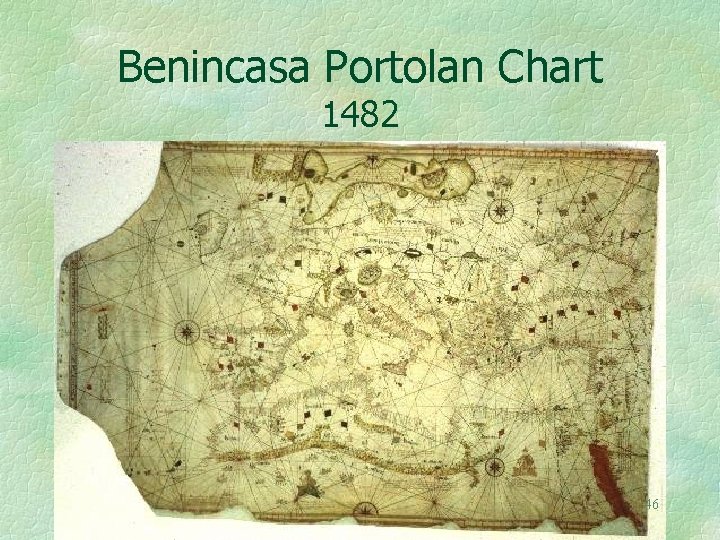
I also have an interest in the structure of old maps. Here is an analysis of one that is over 500 years old. 45

Benincasa Portolan Chart 1482 46

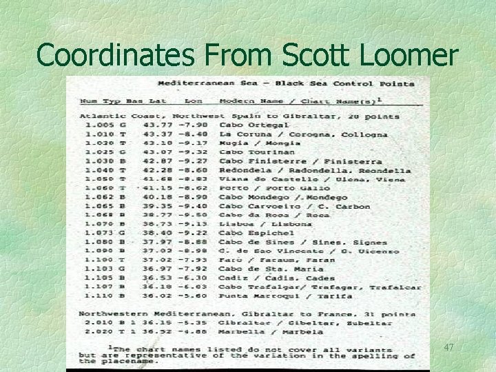
Coordinates From Scott Loomer 47

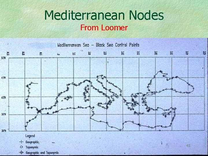
Mediterranean Nodes From Loomer 48

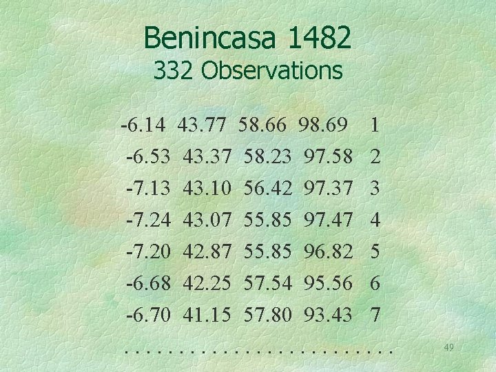
Benincasa 1482 332 Observations -6. 14 43. 77 58. 66 98. 69 1 -6. 53 43. 37 58. 23 97. 58 2 -7. 13 43. 10 56. 42 97. 37 3 -7. 24 43. 07 55. 85 97. 47 4 -7. 20 42. 87 55. 85 96. 82 5 -6. 68 42. 25 57. 54 95. 56 6 -6. 70 41. 15 57. 80 93. 43 7. . . 49

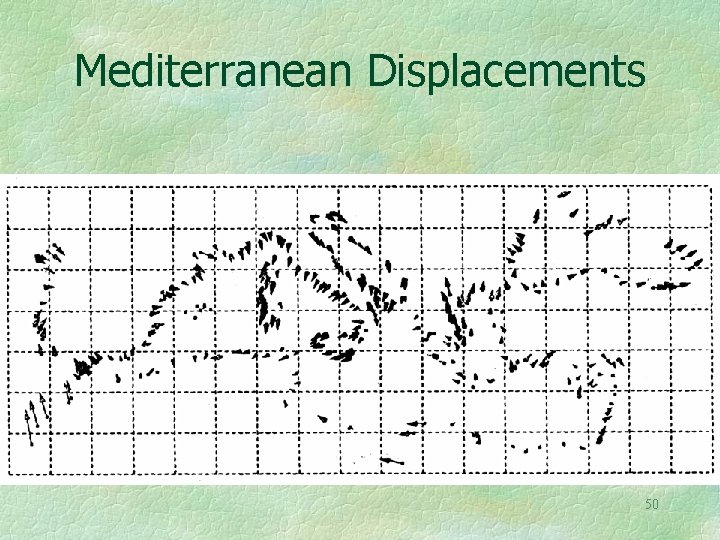
Mediterranean Displacements 50

Interpolated Vector Field Based on Mediterranean displacements 51

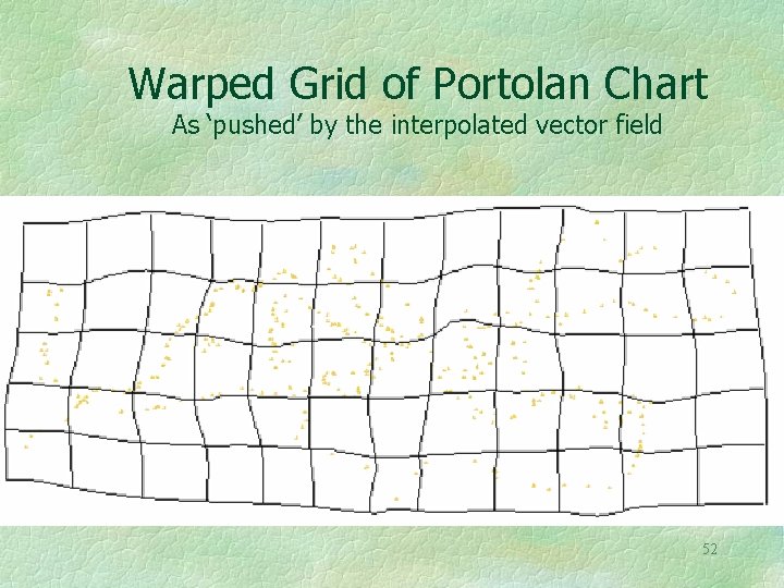
Warped Grid of Portolan Chart As ‘pushed’ by the interpolated vector field 52

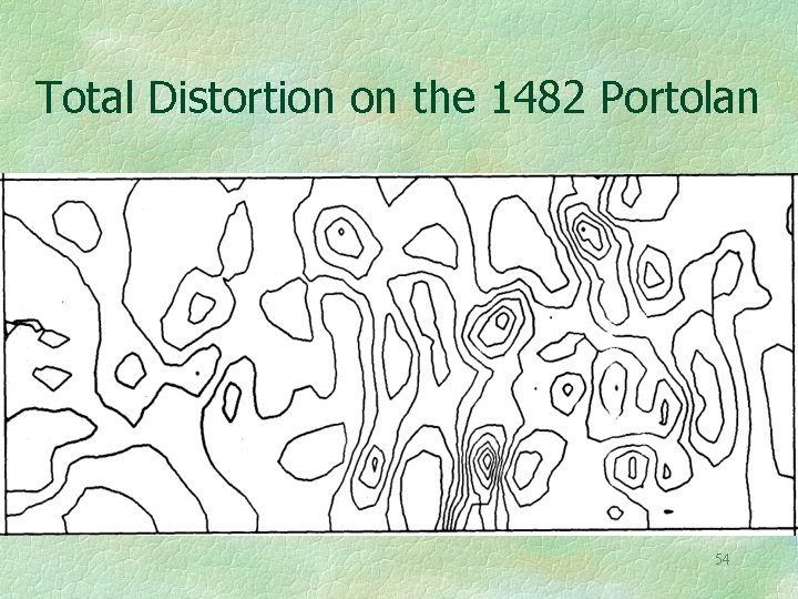
A simple measure of total distortion at each point is the sum of squares of the partial derivatives. This may also be applied to the rubber sheeting shown earlier, or to the migration maps shown later, although in this case the interpretation is more difficult. 53

Total Distortion on the 1482 Portolan 54

Tissot’s Indicatrix also Measures distortion It is based on the four partial derivative of the transformation, u/ x, v/ x, u/ y, v/ y. As such it is a tensor function of location. It varies from place to place, and reflects the fact that map scale is different in every direction at a location, unless the map is conformal. 55

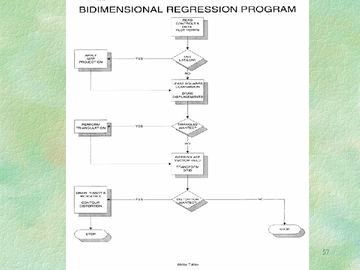
The Coastlines May be Drawn Using the Warped Grid Observe that either the old map, or the modern one, can be considered the independent variable in this bidimensional regression. Relating two sets of coordinates (the old and the new) requires a bidimensional correlation, instead of a regular unidimensional correlation, as did the relation between the student map coordinates and the actual coordinates. The bidimensional correlation can be linear or curvilinear. 56 W. Tobler, 1994, “Bidimensional Regression”, Geographical Analysis, 26 (July): 186 -212

57

Asymmetrical Tables Can Also Lead To Construction Of A Vector Field Start with an asymmetrical geographical table. There are many such tables! It is possible to compute the degree of asymmetry for such tables, and to partition the total variance into symmetric and skew symmetric variances To construct the vector field it is necessary to know the geographic locations and to invoke a model of the 58 process.

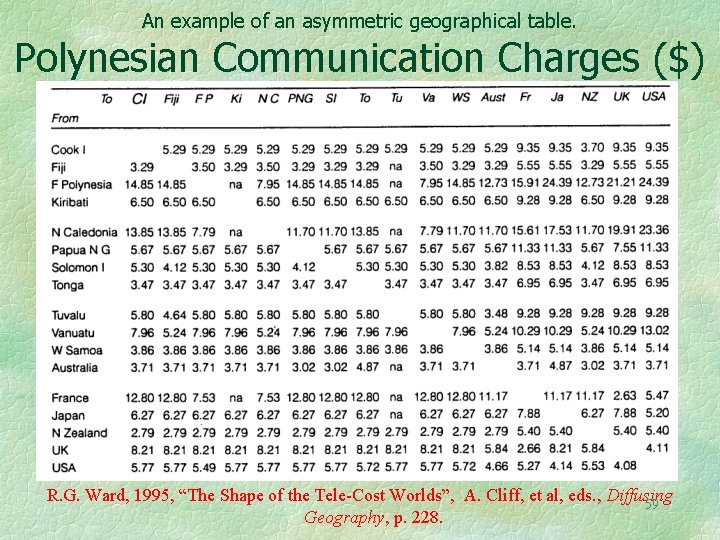
An example of an asymmetric geographical table. Polynesian Communication Charges ($) R. G. Ward, 1995, “The Shape of the Tele-Cost Worlds”, A. Cliff, et al, eds. , Diffusing 59 Geography, p. 228.

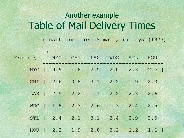
Another example Table of Mail Delivery Times 60

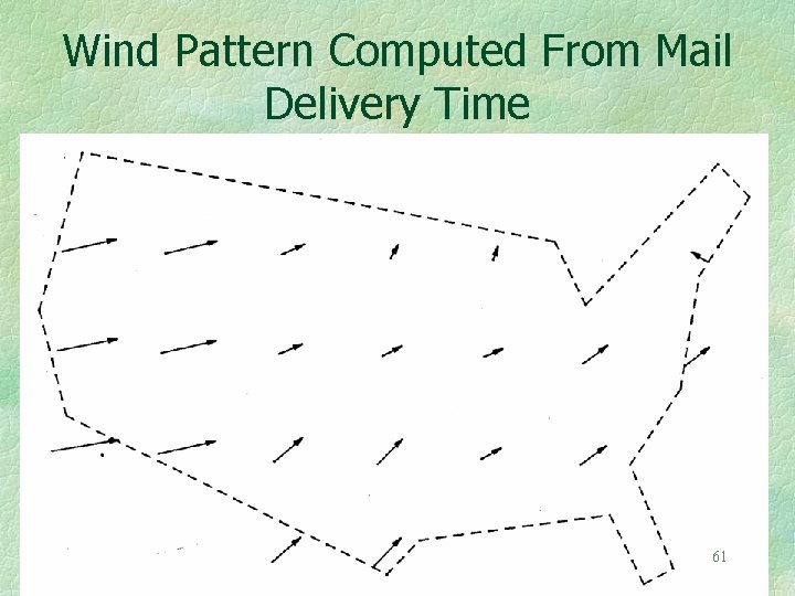
Wind Pattern Computed From Mail Delivery Time 61

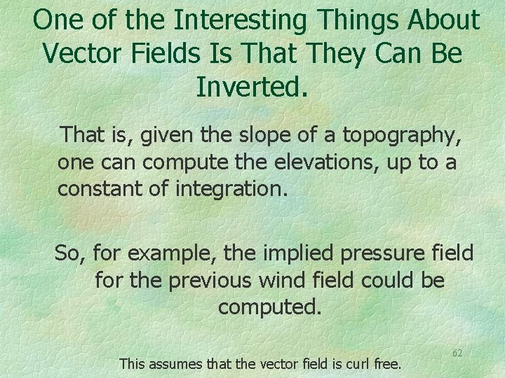
One of the Interesting Things About Vector Fields Is That They Can Be Inverted. That is, given the slope of a topography, one can compute the elevations, up to a constant of integration. So, for example, the implied pressure field for the previous wind field could be computed. This assumes that the vector field is curl free. 62

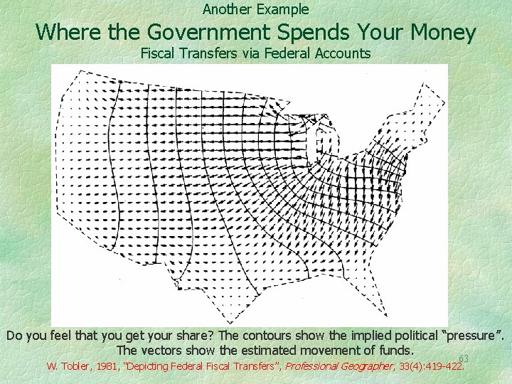
Another Example Where the Government Spends Your Money Fiscal Transfers via Federal Accounts Do you feel that you get your share? The contours show the implied political “pressure”. The vectors show the estimated movement of funds. 63 W. Tobler, 1981, “Depicting Federal Fiscal Transfers”, Professional Geographer, 33(4): 419 -422.

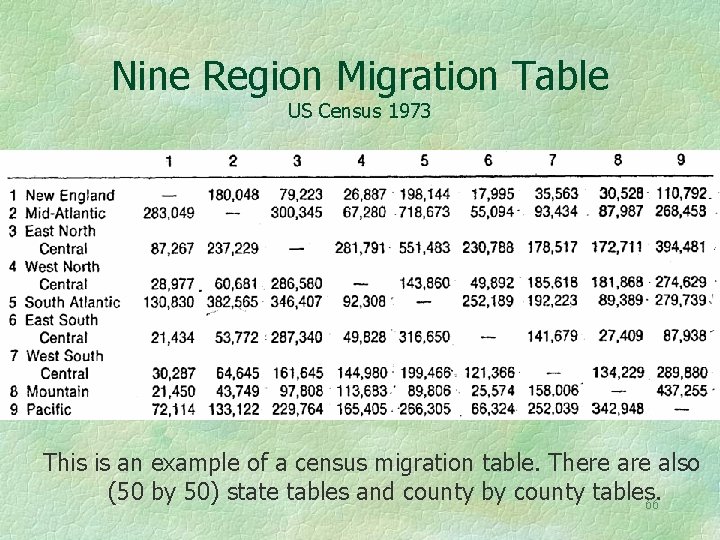
Migration Data Often Come in the Form of Square Tables The rows represent the “from” places and the columns the “to” places. The tables are not symmetrical! 64

A Nine Region US Migration Table Observe that it is not symmetric! Thus there will be places of depletion and places of accumulation! 65

Nine Region Migration Table US Census 1973 This is an example of a census migration table. There also (50 by 50) state tables and county by county tables. 66

There is a great deal of spatial coherence in the migration pattern In the US case the state boundaries hide the effect, as would the county boundaries in the UK case. Therefore they are omitted. There is also temporal coherence. W. Tobler, 1995, “Migration: Ravenstein, Thornthwaite, and Beyond”, Urban 67 Geography, 16(4): 327 -343.

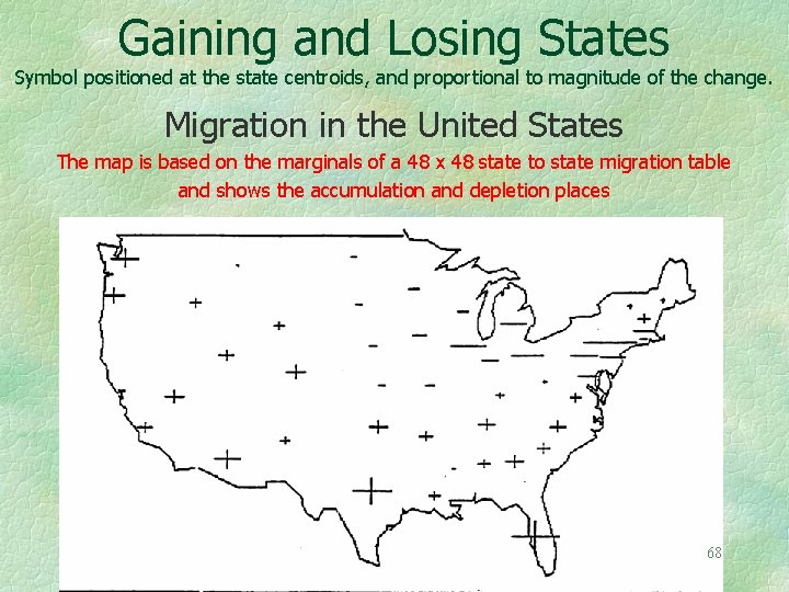
Gaining and Losing States Symbol positioned at the state centroids, and proportional to magnitude of the change. Migration in the United States The map is based on the marginals of a 48 x 48 state to state migration table and shows the accumulation and depletion places 68

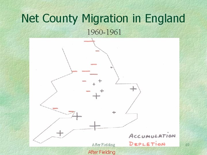
Net County Migration in England 1960 -1961 After Fielding 69

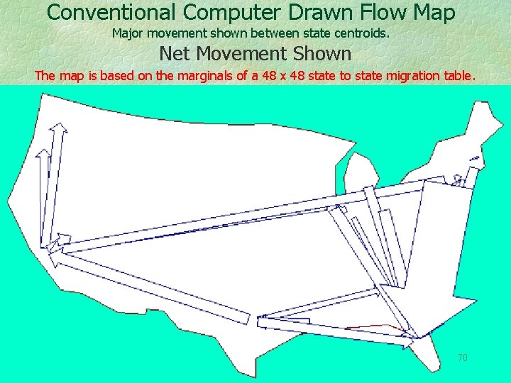
Conventional Computer Drawn Flow Map Major movement shown between state centroids. Net Movement Shown The map is based on the marginals of a 48 x 48 state to state migration table. 70

Notice that only the Net Movements from the Table are being used These are the difference of the marginals. In-movement minus out-movement. From the asymmetry of the table margins one can compute an attractivity, or pressure to move. Of course this requires a model. G. Dorigo, & Tobler, W. , 1983, “Push-Pull Migration Laws”, Annals, AAG, 7391): 1 -17. 71

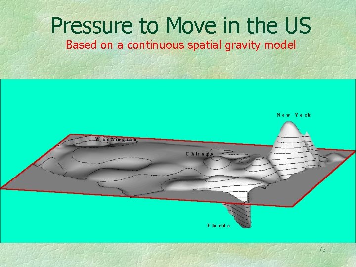
Pressure to Move in the US Based on a continuous spatial gravity model 72

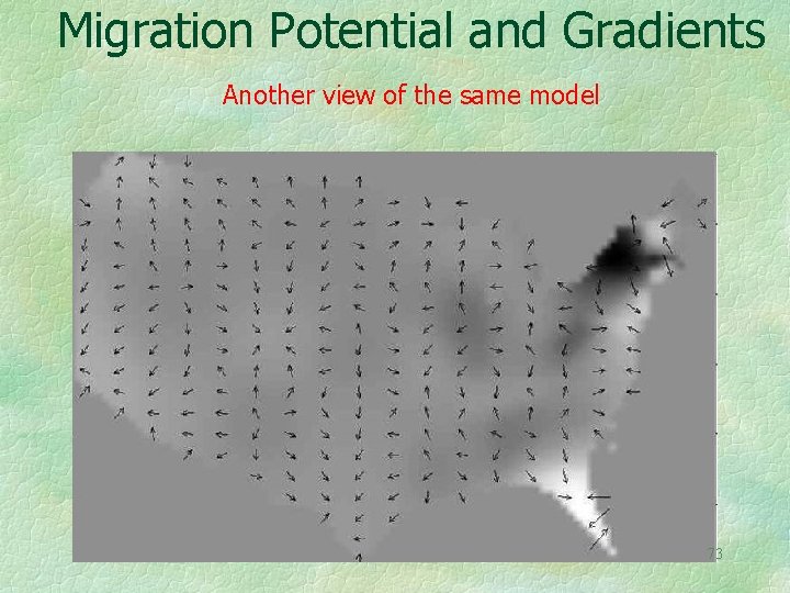
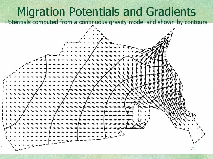
Migration Potential and Gradients Another view of the same model 73

Migration Potentials and Gradients Potentials computed from a continuous gravity model and shown by contours 74

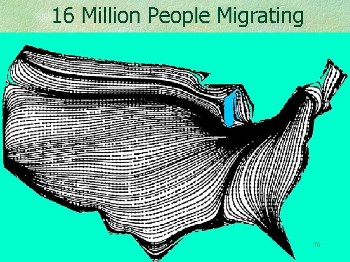
Recall that several million people migrate during the 5 year census period The next map shows an ensemble average, not the path of any individual. But observe, not unrealistically, that the people to the East of Detroit tend to go to the Southeast, and Minnesotans to the Northwest, and the 75 remainder to the Southwest.

16 Million People Migrating 76

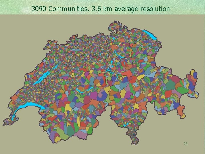
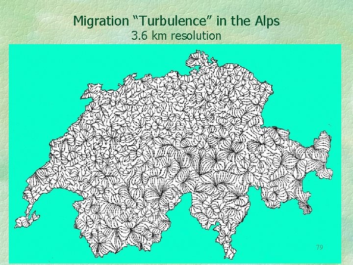
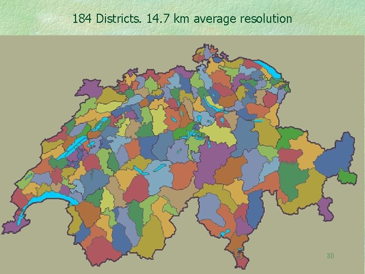
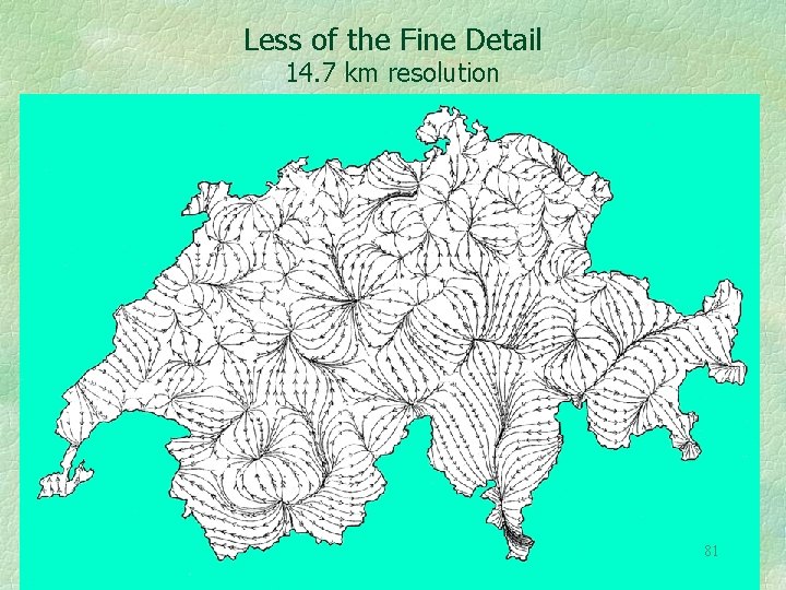
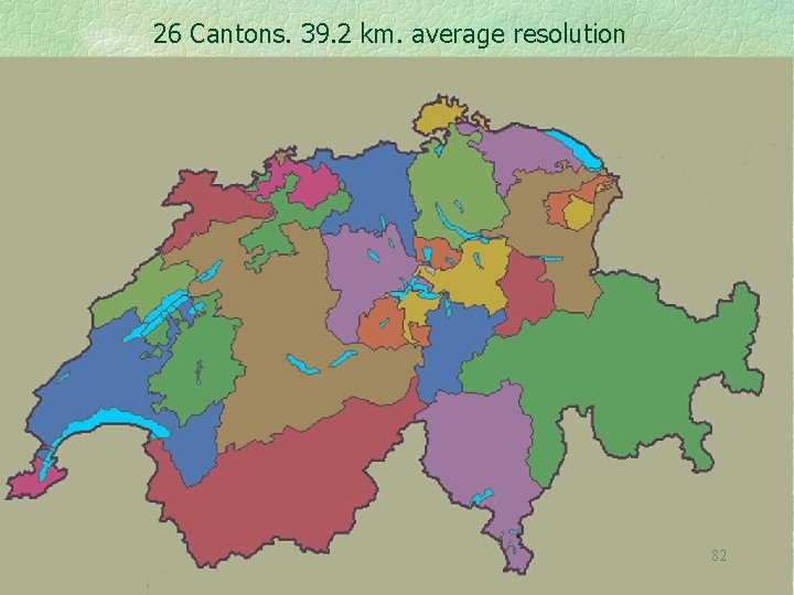
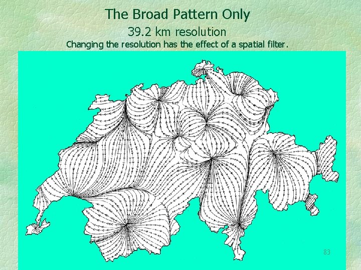
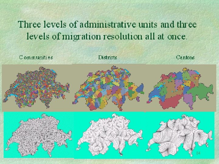
Changing the resolution acts as a spatial filter. This is shown by vector fields at several levels of resolution. The next several maps are of net migration in Switzerland. 3. 6 km resolution (3090 Gemeinde) 14. 7 km resolution (184 Bezirke) 39. 2 km resolution (26 Kantone ) Maps by Guido Dorigo, University of Zürich 77

3090 Communities. 3. 6 km average resolution 78

Migration “Turbulence” in the Alps 3. 6 km resolution 79

184 Districts. 14. 7 km average resolution 80

Less of the Fine Detail 14. 7 km resolution 81

26 Cantons. 39. 2 km. average resolution 82

The Broad Pattern Only 39. 2 km resolution Changing the resolution has the effect of a spatial filter. 83

84

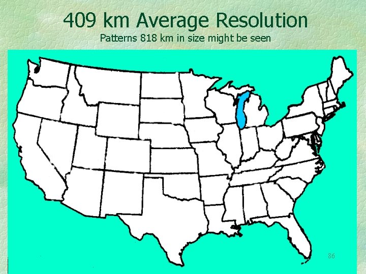
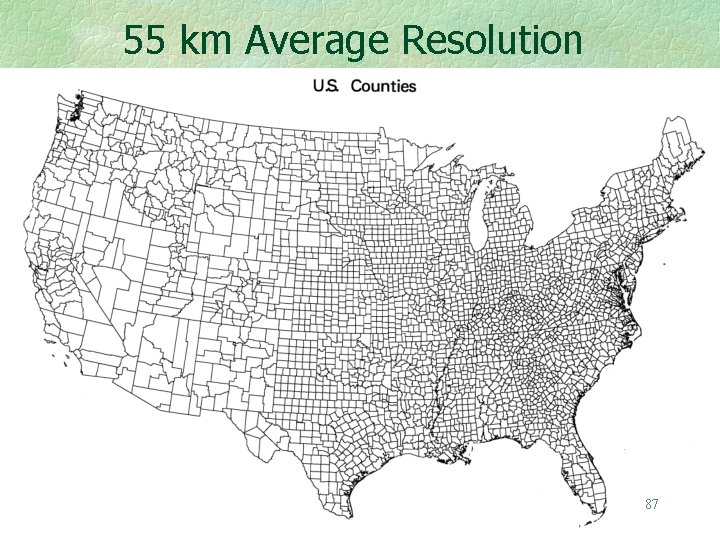
Some consequences of Resolution for Movement Studies. A State to State migration table yields a 50 by 50 migration table, with 2, 500 entries. Patterns as small as 800 km in extent might be seen. A county to county migration table 3141 by 3141 in size could contain over 9 million entries. (It actually contains only 5% of these). A table of worldwide movement or trade between all countries could contain nearly 40, 000 numbers. This is why most statistical almanacs do not contain from-to tables. 85

409 km Average Resolution Patterns 818 km in size might be seen 86

55 km Average Resolution 87

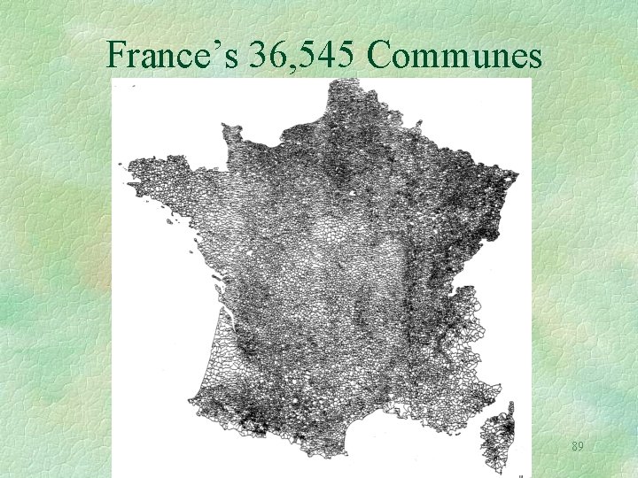
Think Big! The 36, 000 communes of France could yield a migration or interaction table with as many as 1, 335, 537, 025 entries. (3 km average resolution) 88

France’s 36, 545 Communes 89

A table giving the interaction of everybody on earth with everyone else would be 6 x 109 by 6 x 109 in size, and that’s only for one time interval! But it is a very sparse table, each person having at most a few thousand connections. 90

In Summary I have proceeded from very simple topographic slopes to movement models, using a variety of vector fields. In case you wish to go furthere is appended a short list of books that I have found useful. 91

J. Marsen, & Tromba, A. , 1988, Vector Calculus, 3 rd ed. , Freeman, New York. R. Osserman, 1968, Two Dimensional Calculus, Harcourt Brace, New York. H. Schey, 1975, Div, Grad, Curl, and all That, 1 st ed. , Norton, New York. 92

Thank you for your attention. 93