The binomial applied absolute and relative risks chisquare

The binomial applied: absolute and relative risks, chi-square

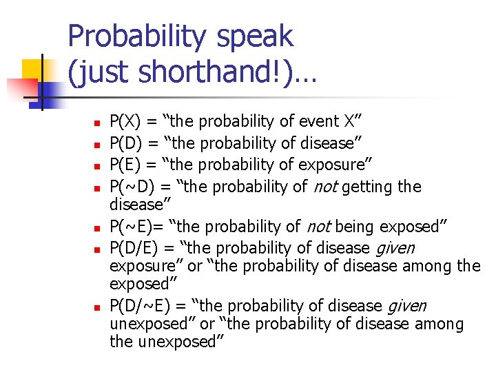
Probability speak (just shorthand!)… n n n n P(X) = “the probability of event X” P(D) = “the probability of disease” P(E) = “the probability of exposure” P(~D) = “the probability of not getting the disease” P(~E)= “the probability of not being exposed” P(D/E) = “the probability of disease given exposure” or “the probability of disease among the exposed” P(D/~E) = “the probability of disease given unexposed” or “the probability of disease among the unexposed”

Things that follow a binomial distribution… Cohort study (or cross-sectional): n n The number of exposed individuals in your sample that develop the disease The number of unexposed individuals in your sample that develop the disease Case-control study: n n The number of cases that have had the exposure The number of controls that have had the exposure

Cohort study example: n You sample 100 smokers and 100 nonsmokers and follow them for 5 years to see who develops heart disease.

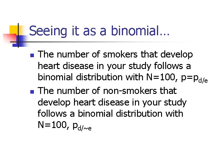
Seeing it as a binomial… n n The number of smokers that develop heart disease in your study follows a binomial distribution with N=100, p=pd/e The number of non-smokers that develop heart disease in your study follows a binomial distribution with N=100, pd/~e

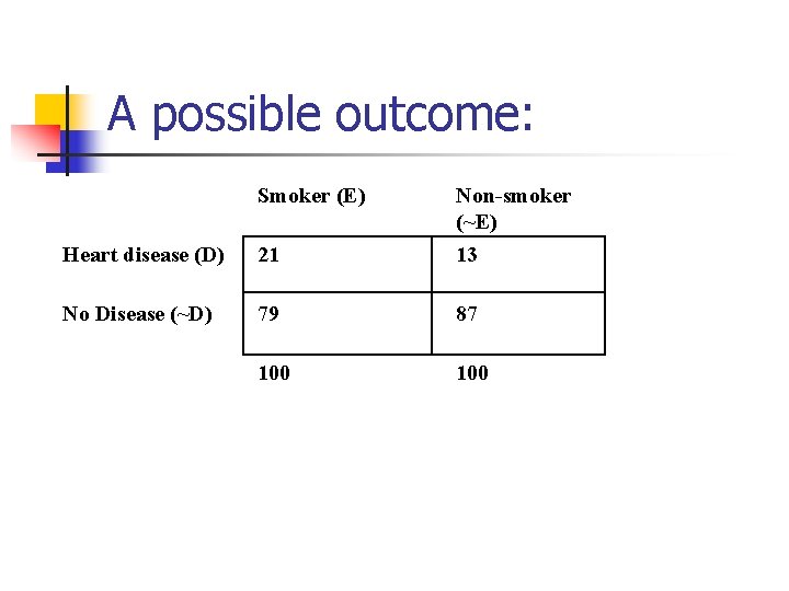
A possible outcome: Smoker (E) Heart disease (D) 21 Non-smoker (~E) 13 No Disease (~D) 79 87 100

Statistics for these data n n n 1. Risk ratio (relative risk) 2. Difference in proportions (absolute risk) 3. Chi-square test of independence n For 2 x 2 tables, mathematically equivalent to difference in proportions Z test.

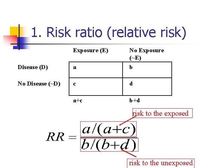
1. Risk ratio (relative risk) Exposure (E) Disease (D) a No Exposure (~E) b No Disease (~D) c d a+c b+d risk to the exposed risk to the unexposed

In probability terms… Exposure (E) Disease (D) a No Exposure (~E) b No Disease (~D) c d a+c b+d Risk of disease in the exposed risk of disease in the unexposed

Risk ratio calculation: Smoker (E) Heart disease (D) 21 Non-smoker (~E) 13 No Disease (~D) 79 87 100 Interpretation: there is a 61% increase in risk of heart disease in smokers vs. nonsmokers n

Inferences about risk ratio… n n n Is our observed risk ratio statistically different from 1. 0? What is the p-value? I’m going to present statistical inference for odds ratio; risk ratio is similar. So, for now, just get answer from SAS: n n 95% confidence interval: 0. 86 to 3. 04 P-value>. 05

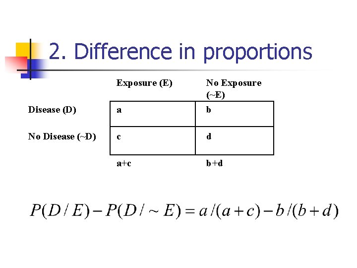
2. Difference in proportions Exposure (E) Disease (D) a No Exposure (~E) b No Disease (~D) c d a+c b+d

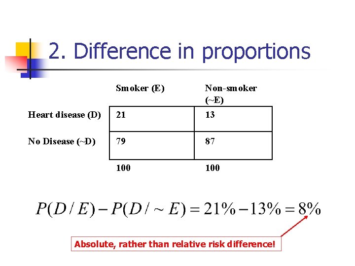
2. Difference in proportions Smoker (E) Heart disease (D) 21 Non-smoker (~E) 13 No Disease (~D) 79 87 100 Absolute, rather than relative risk difference!

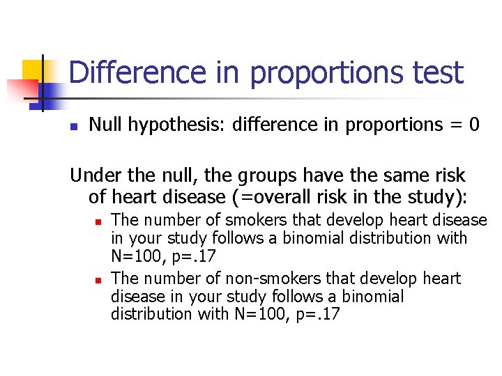
Difference in proportions test n Null hypothesis: difference in proportions = 0 Under the null, the groups have the same risk of heart disease (=overall risk in the study): n n The number of smokers that develop heart disease in your study follows a binomial distribution with N=100, p=. 17 The number of non-smokers that develop heart disease in your study follows a binomial distribution with N=100, p=. 17

Follows a normal because binomial can be approximated with normal Difference in proportions test Null hypothesis: The difference in proportions is 0. Recall, variance of a proportion is p(1 -p)/n Use average (or pooled) proportion in standard error formula, because under the null hypothesis, groups have equal proportions.

Z-test applied here… Corresponding two-sided p-value is. 131.

Corresponding 95% confidence interval… If the 95% confidence interval crosses the null value (here=0), then p>. 05

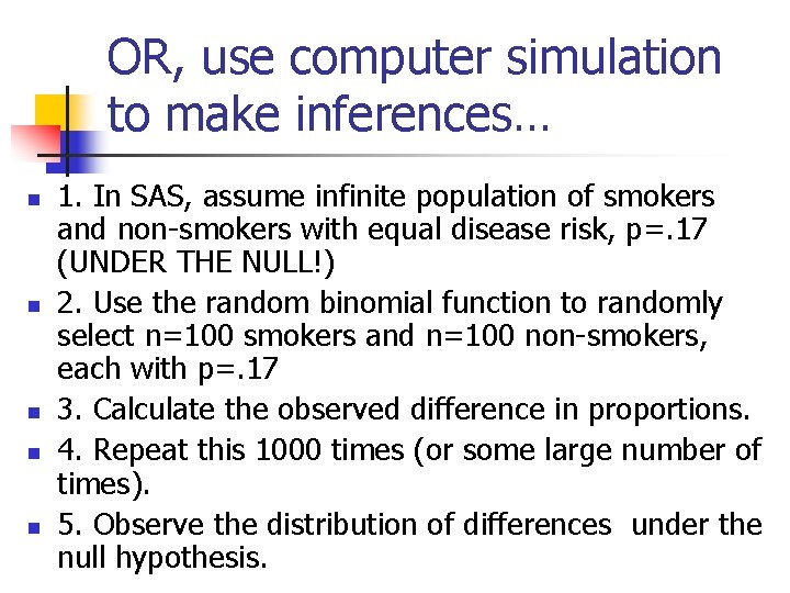
OR, use computer simulation to make inferences… n n n 1. In SAS, assume infinite population of smokers and non-smokers with equal disease risk, p=. 17 (UNDER THE NULL!) 2. Use the random binomial function to randomly select n=100 smokers and n=100 non-smokers, each with p=. 17 3. Calculate the observed difference in proportions. 4. Repeat this 1000 times (or some large number of times). 5. Observe the distribution of differences under the null hypothesis.

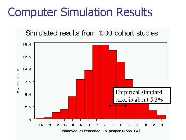
Computer Simulation Results Empirical standard error is about 5. 3%

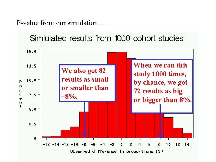
P-value from our simulation… We also got 82 results as small or smaller than – 8%. When we ran this study 1000 times, by chance, we got 72 results as big or bigger than 8%.

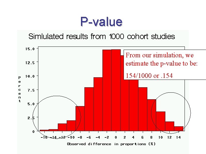
P-value From our simulation, we estimate the p-value to be: 154/1000 or. 154

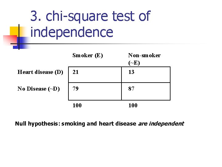
3. chi-square test of independence Smoker (E) Heart disease (D) 21 Non-smoker (~E) 13 No Disease (~D) 79 87 100 Null hypothesis: smoking and heart disease are independent

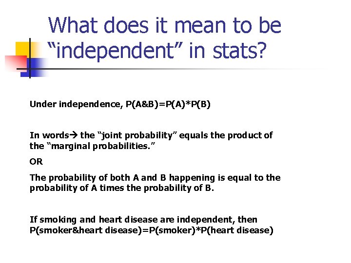
What does it mean to be “independent” in stats? Under independence, P(A&B)=P(A)*P(B) In words the “joint probability” equals the product of the “marginal probabilities. ” OR The probability of both A and B happening is equal to the probability of A times the probability of B. If smoking and heart disease are independent, then P(smoker&heart disease)=P(smoker)*P(heart disease)

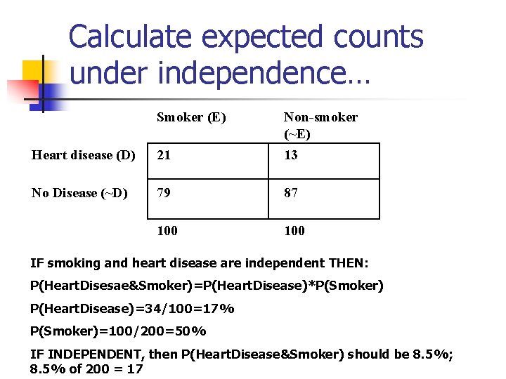
Calculate expected counts under independence… Smoker (E) Heart disease (D) 21 Non-smoker (~E) 13 No Disease (~D) 79 87 100 IF smoking and heart disease are independent THEN: P(Heart. Disesae&Smoker)=P(Heart. Disease)*P(Smoker) P(Heart. Disease)=34/100=17% P(Smoker)=100/200=50% IF INDEPENDENT, then P(Heart. Disease&Smoker) should be 8. 5%; 8. 5% of 200 = 17

Fill in the expected table… Smoker (E) Heart disease (D) 17 No Disease (~D) 83 100 Non-smoker (~E) Marginals are fixed! 17 34 83 156 100 Notice that the rest of the table is determined after you fill in 17 for cell A. There are no degrees of freedom left! (This table has only 1 degree of freedom).

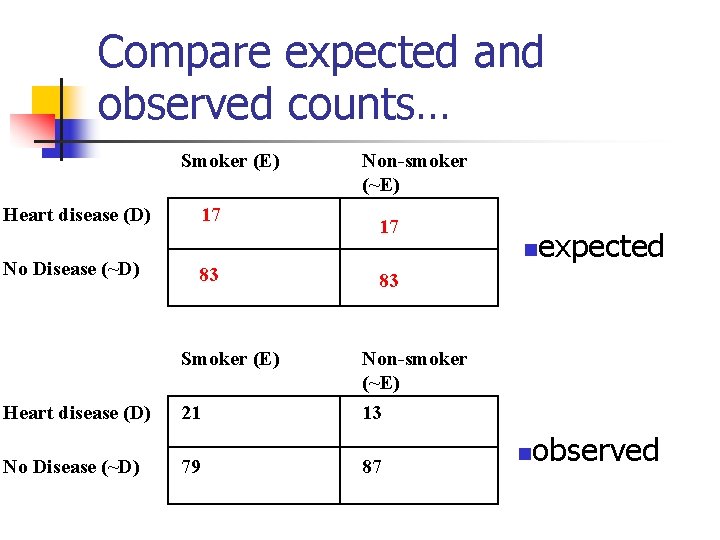
Compare expected and observed counts… Smoker (E) Heart disease (D) 17 No Disease (~D) Non-smoker (~E) 17 n 83 expected 83 Smoker (E) Heart disease (D) 21 Non-smoker (~E) 13 No Disease (~D) 79 87 n observed

Chi-Square test 2. 25=1. 5 squared. The chi-square test produces exactly the square of the Z-test and the same p-value. Degrees of freedom = (rows-1)*(columns-1)=(2 -1)*(2 -1)=1 Rule of thumb: if the chi-square statistic is much greater than it’s degrees of freedom, indicates statistical significance. Here 2. 25 not quite big enough—p=. 131.

Bonus material: The Chi-Square distribution: is sum of squared normal deviates The expected value and variance of a chi-square: E(x)=df Var(x)=2(df)

Case-control study example: n You sample 50 stroke patients and 50 controls without stroke and ask about their smoking in the past.

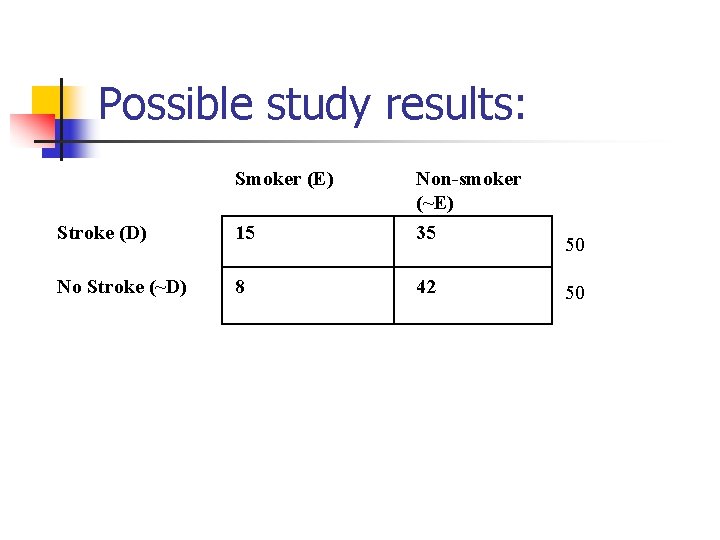
Possible study results: Smoker (E) Stroke (D) 15 Non-smoker (~E) 35 No Stroke (~D) 8 42 50 50

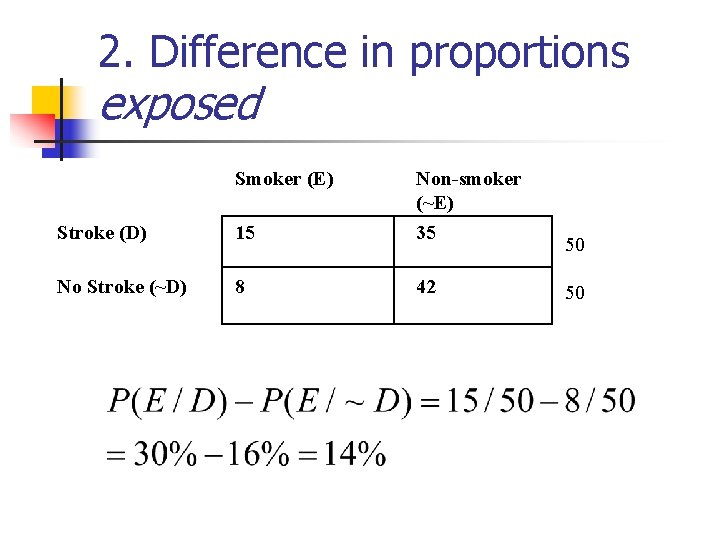
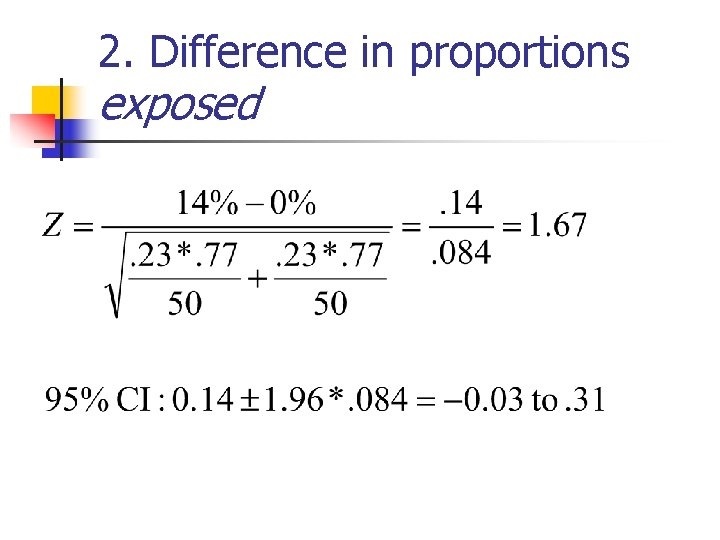
Statistics for these data n n n 1. Odds ratio (relative risk) 2. Difference in proportions exposed (absolute risk) 3. Chi-square

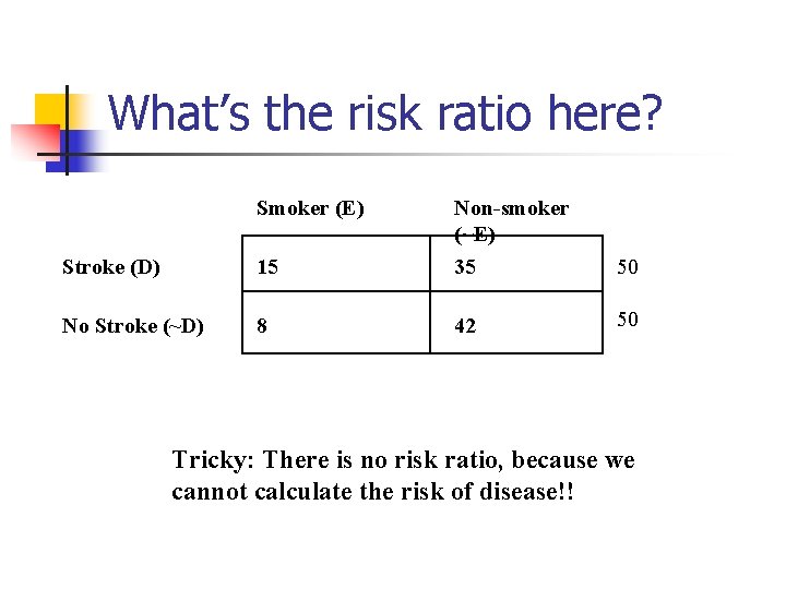
What’s the risk ratio here? Smoker (E) 15 Non-smoker (~E) 35 Stroke (D) No Stroke (~D) 50 8 42 50 Tricky: There is no risk ratio, because we cannot calculate the risk of disease!!

The odds ratio… n We cannot calculate a risk ratio from a case-control study. n BUT, we can calculate a measure called the odds ratio…

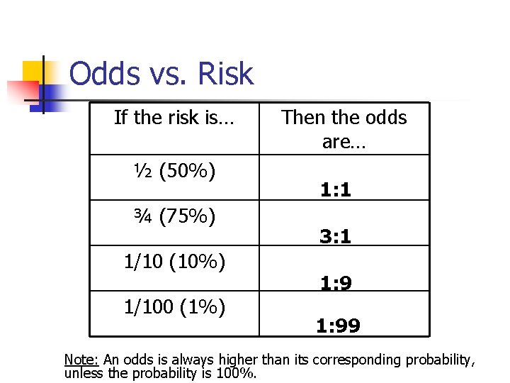
Odds vs. Risk If the risk is… ½ (50%) ¾ (75%) 1/10 (10%) 1/100 (1%) Then the odds are… 1: 1 3: 1 1: 99 Note: An odds is always higher than its corresponding probability, unless the probability is 100%.

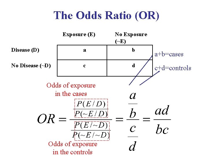
The Odds Ratio (OR) Exposure (E) Disease (D) a No Disease (~D) c No Exposure (~E) b d Odds of exposure in. The theproportion cases of cases to controls are set by the investigator; therefore, they do not represent the risk (probability) of developing disease. Odds of exposure in the controls a+b=cases c+d=controls

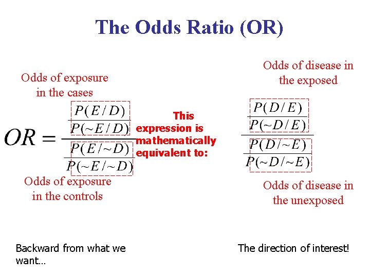
The Odds Ratio (OR) Odds of disease in the exposed Odds of exposure in the cases This expression is mathematically equivalent to: Odds of exposure in the controls Backward from what we want… Odds of disease in the unexposed The direction of interest!

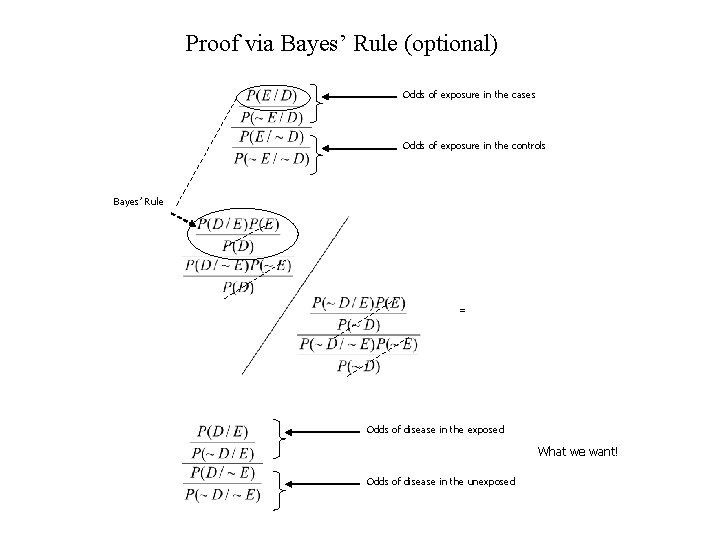
Proof via Bayes’ Rule (optional) Odds of exposure in the cases Odds of exposure in the controls Bayes’ Rule = Odds of disease in the exposed What we want! Odds of disease in the unexposed

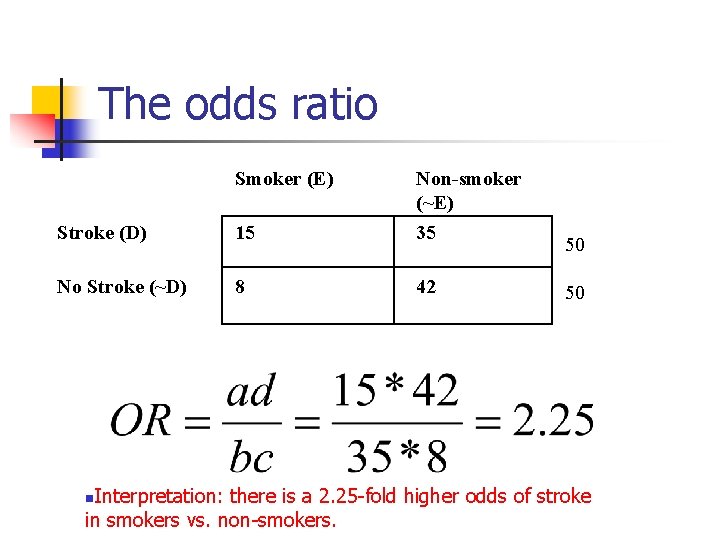
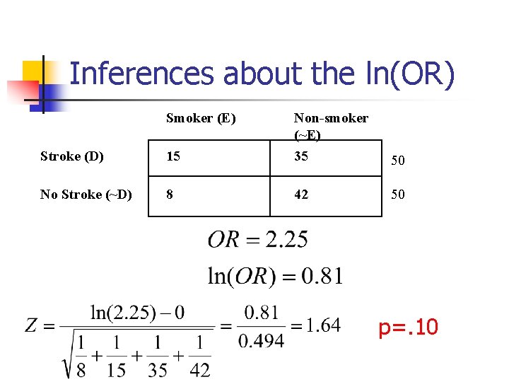
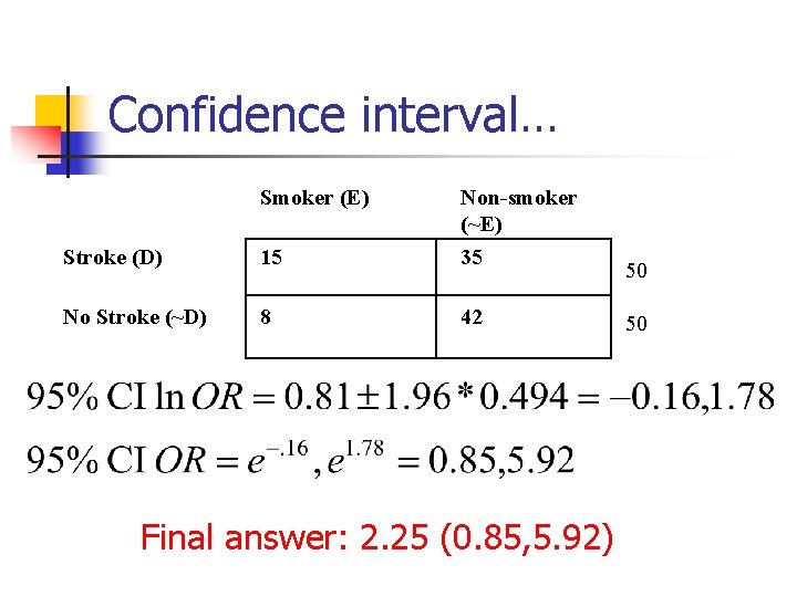
The odds ratio Smoker (E) Stroke (D) 15 Non-smoker (~E) 35 No Stroke (~D) 8 42 50 50 Interpretation: there is a 2. 25 -fold higher odds of stroke in smokers vs. non-smokers. n

Inferences about the odds ratio… n n Does the sampling distribution follow a normal distribution? What is the standard error?

Simulation… n n n 1. In SAS, assume infinite population of cases and controls with equal proportion of smokers (exposure), p=. 23 (UNDER THE NULL!) 2. Use the random binomial function to randomly select n=50 cases and n=50 controls each with p=. 23 chance of being a smoker. 3. Calculate the observed odds ratio for the resulting 2 x 2 table. 4. Repeat this 1000 times (or some large number of times). 5. Observe the distribution of odds ratios under the null hypothesis.

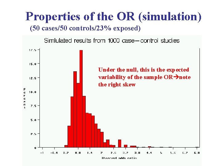
Properties of the OR (simulation) (50 cases/50 controls/23% exposed) Under the null, this is the expected variability of the sample OR note the right skew

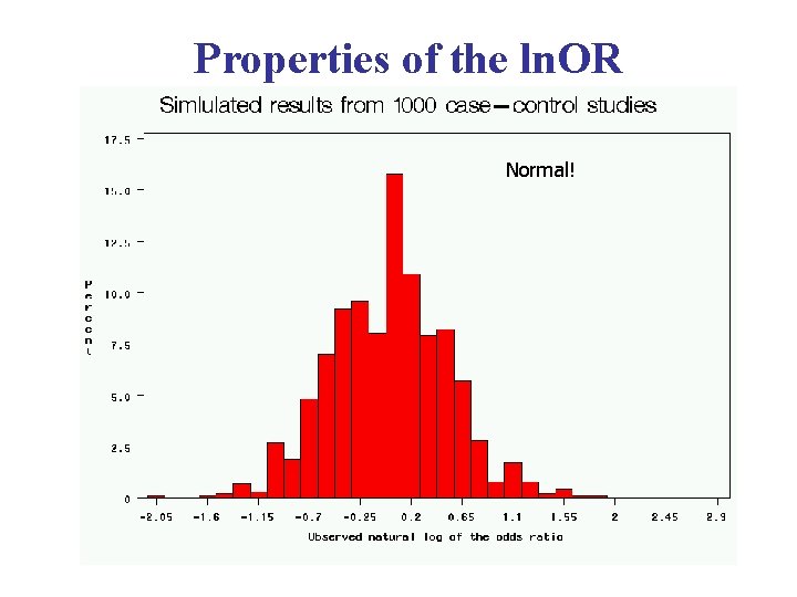
Properties of the ln. OR Normal!

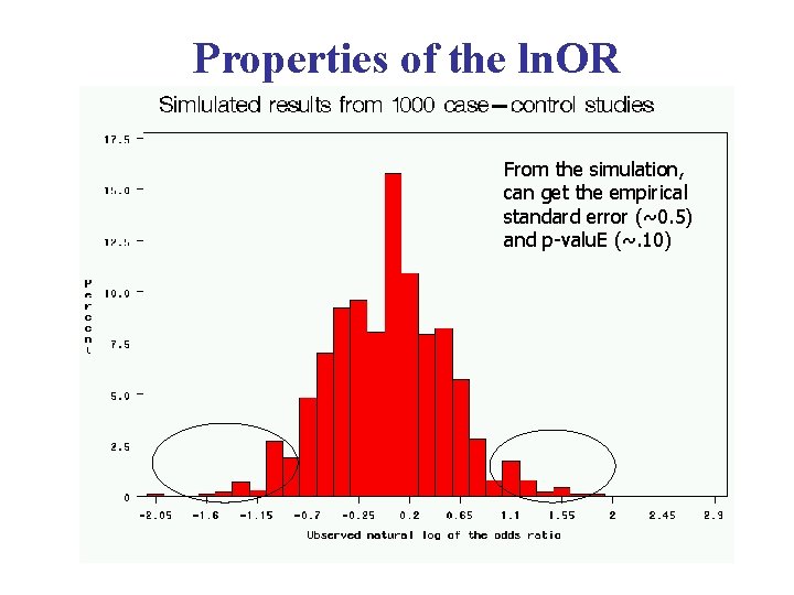
Properties of the ln. OR From the simulation, can get the empirical standard error (~0. 5) and p-valu. E (~. 10)

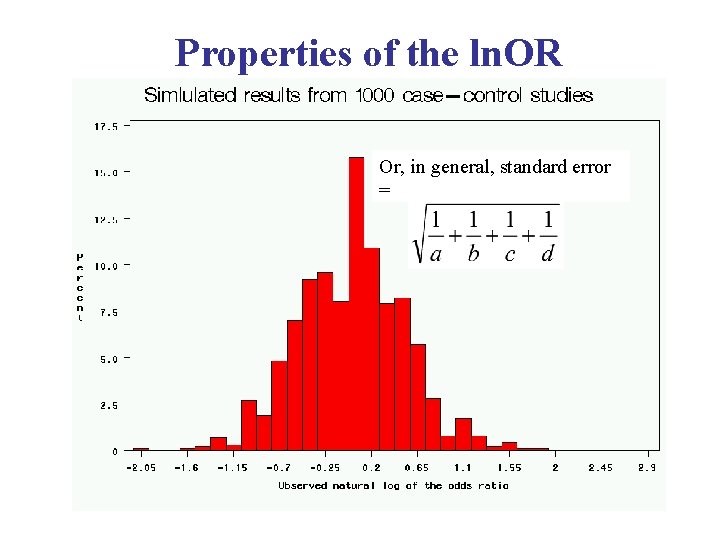
Properties of the ln. OR Or, in general, standard error =

Inferences about the ln(OR) Smoker (E) 15 Non-smoker (~E) 35 Stroke (D) No Stroke (~D) 50 8 42 50 p=. 10

Confidence interval… Smoker (E) Stroke (D) 15 Non-smoker (~E) 35 No Stroke (~D) 8 42 Final answer: 2. 25 (0. 85, 5. 92) 50 50

2. Difference in proportions exposed Smoker (E) Stroke (D) 15 Non-smoker (~E) 35 No Stroke (~D) 8 42 50 50

2. Difference in proportions exposed

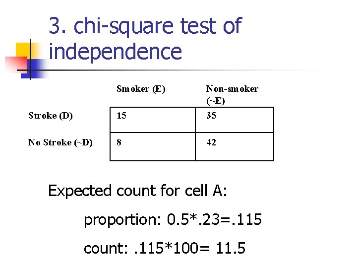
3. chi-square test of independence Smoker (E) Stroke (D) 15 Non-smoker (~E) 35 No Stroke (~D) 8 42 Expected count for cell A: proportion: 0. 5*. 23=. 115 count: . 115*100= 11. 5

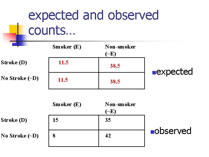
expected and observed counts… Smoker (E) Stroke (D) 11. 5 Non-smoker (~E) 38. 5 n No Stroke (~D) 11. 5 expected 38. 5 Smoker (E) Stroke (D) 15 Non-smoker (~E) 35 No Stroke (~D) 8 42 n observed

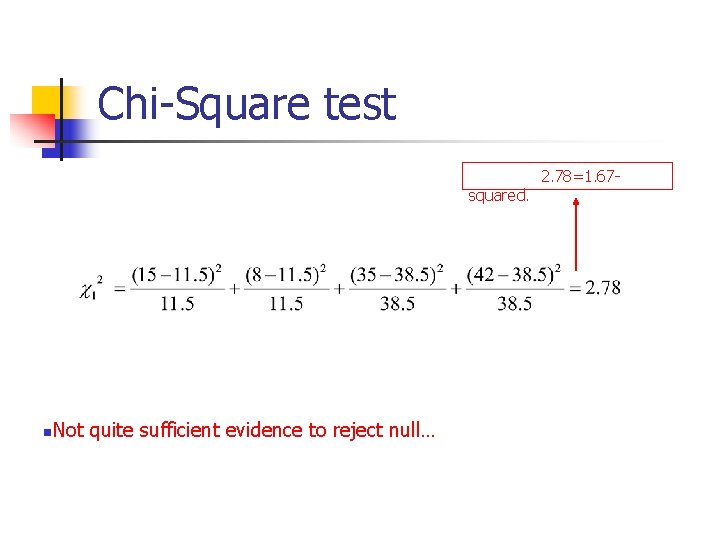
Chi-Square test squared. n Not quite sufficient evidence to reject null… 2. 78=1. 67 -