The Basics of Structural Equation Modeling James G

The Basics of Structural Equation Modeling James G. Anderson, Ph. D. Purdue University

Objective • To confirm a theory involving hypotheses concerning the causal relations that generate covariation among a set of observed variables.

Structural Equation Modeling • Hypothetical structural relations among concepts are represented pictorially with a path diagram • The causal processes under study are represented with a set of structural (i. e. , regression) equations

Structural Equation Modeling • The hypothesized model is tested statistically in a simultaneous analysis of the entire system of variables to determine the degree to which it is consistent with the data. • If the goodness-of-fit of the model to the data is adequate, the postulated relations among the variables are considered to be plausible. • If the goodness-of-fit is inadequate, the postulated relations among the variables are rejected.

Comparison of SEM to Other Multivariate Statistical Procedures (MSP) • SEM is confirmatory; most MSP are exploratory so that hypothesis testing is difficult. SEM provides estimates of measurement parameter; MSP are incapable of assessing or correcting for measurement error. SEM can incorporate both obser • ved and unobserved (i. e. , latent) variables; MSP are based only on observed variables.

The SEM Process Specification of theoretical (causal) model • Path diagram • Exogenous variables • Endogenous variables

Example: Theory of Reasoned Action

Data Collection • The theoretical concepts must be operationalized and data collected. • Sample size should be >100, preferably >200 • In general the ratio of sample size to estimated parameter should be at least 10: 1.

Model Specification • Measurement model • Structural model

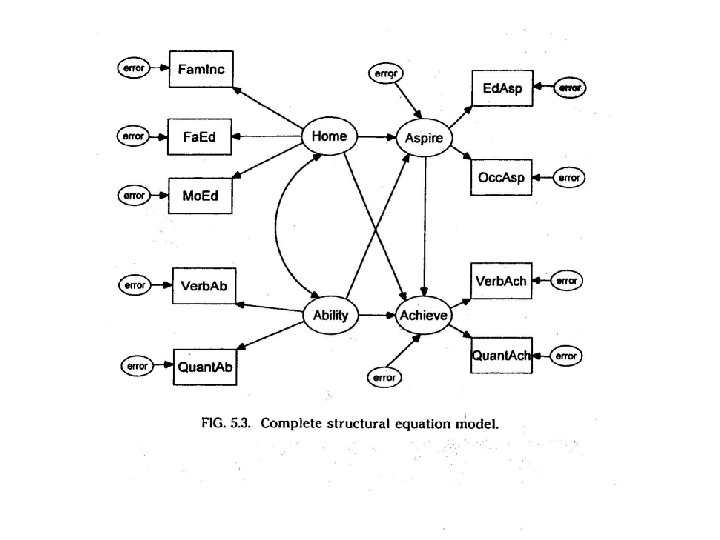
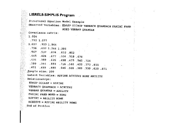
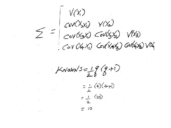
Identification • You cannot estimate more parameters than the number of unique elements in the covariance matrix, k(k-1)/2. • Identification is achieved by placing restrictions on the model parameters.

Parameter Estimation • Fit Criteria OLS = tr (S-C)2 GLS = 1/2 tr [(S-C)S-1]2 ML = ln|C| - In|S| + tr SC-1 - m tr=trace (sum of the diagonal elements), S=covariance matrix implied by the model, C= observed covariance matrix, ln=natural logarithm, | | indicates the determinant of the matrix. m= total number of variables

Testing the Goodness-of-Fit • Data = Model Predictions + Residual • (N-1)Fmin is distributed as chi square with df = 1/2 (p)(p+1) - t p = no. of observed variables t = no. of parameters estimated • Fmin is the minimum value of the fit function • N = the total number of observations

Model Modification • • Modification indices Residuals Difference in Chi square Replication of the model with an independent data set

Inferences from the Model

Potential Problems • Inadequate theory • Data that violates the assumptions • Failure to examine the possibility of interaction effects • Model building not based on theoretically justified relations among variables

Potential Problems • Failure to distinguish between inductive and deductive model building. • Causal inferences from the analysis • Poor reporting of the results