The Automatic Generation of Mutation Operators pptx for

The Automatic Generation of Mutation. Operators. pptx for Genetic Algorithms [Workshop on Evolutionary Computation for the Automated Design of Algorithms 2012] John Woodward – Nottingham (CHINA) Jerry Swan - Stirling 1

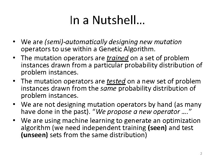
In a Nutshell… • We are (semi)-automatically designing new mutation operators to use within a Genetic Algorithm. • The mutation operators are trained on a set of problem instances drawn from a particular probability distribution of problem instances. • The mutation operators are tested on a new set of problem instances drawn from the same probability distribution of problem instances. • We are not designing mutation operators by hand (as many have done in the past). “We propose a new operator …. ” • We are using machine learning to generate an optimization algorithm (we need independent training (seen) and test (unseen) sets from the same distribution) 2

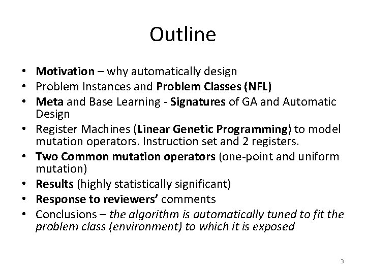
Outline • Motivation – why automatically design • Problem Instances and Problem Classes (NFL) • Meta and Base Learning - Signatures of GA and Automatic Design • Register Machines (Linear Genetic Programming) to model mutation operators. Instruction set and 2 registers. • Two Common mutation operators (one-point and uniform mutation) • Results (highly statistically significant) • Response to reviewers’ comments • Conclusions – the algorithm is automatically tuned to fit the problem class (environment) to which it is exposed 3

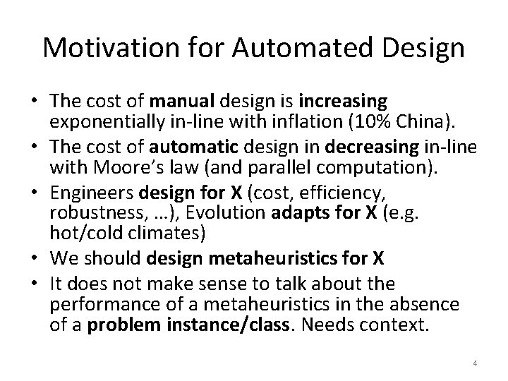
Motivation for Automated Design • The cost of manual design is increasing exponentially in-line with inflation (10% China). • The cost of automatic design in decreasing in-line with Moore’s law (and parallel computation). • Engineers design for X (cost, efficiency, robustness, …), Evolution adapts for X (e. g. hot/cold climates) • We should design metaheuristics for X • It does not make sense to talk about the performance of a metaheuristics in the absence of a problem instance/class. Needs context. 4

Problem Instances and Classes A problem instance is a single example of an optimization problem (in this paper either a realvalued function defined over 32 or 64 bits). A problem class is a probability distribution over problem instances. Often we do not have explicit access to the probability distribution but we can only sample it (except with synthetic problems). 5

Important Consequence of No Free Lunch (NFL) Theorems • Loosely, NFL states under a uniform probability distribution over problem instances, all metaheuristics perform equally well (in fact identically). It formalizes a trade-off. • This implies that under some other distributions (in fact ‘almost all’), some algorithms will be superior. • Automatic design can exploit the fact an assumption of NFL is not valid (which is the case with most real world applications). 6

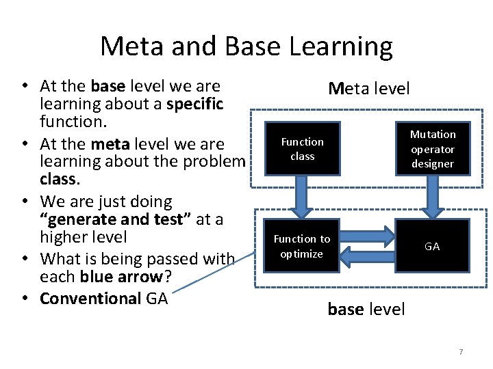
Meta and Base Learning • At the base level we are learning about a specific function. • At the meta level we are learning about the problem class. • We are just doing “generate and test” at a higher level • What is being passed with each blue arrow? • Conventional GA Meta level Function class Mutation operator designer Function to optimize GA base level 7

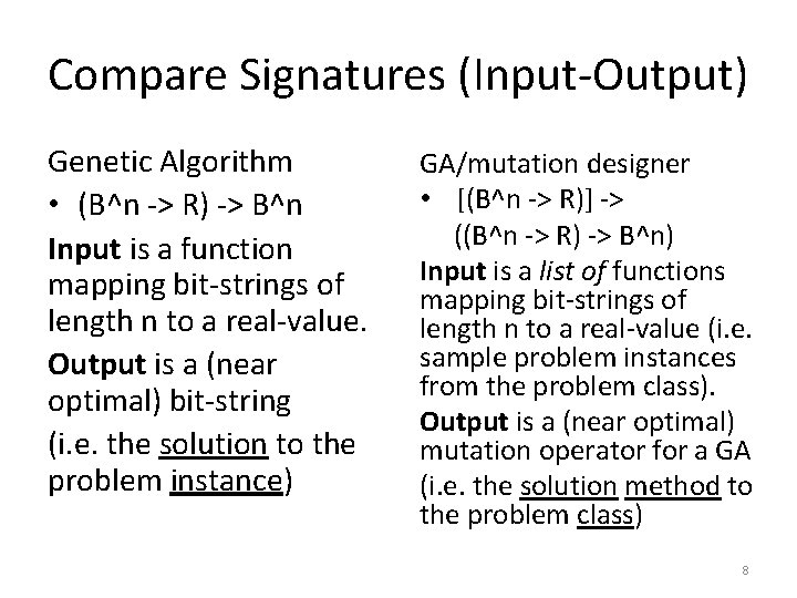
Compare Signatures (Input-Output) Genetic Algorithm • (B^n -> R) -> B^n Input is a function mapping bit-strings of length n to a real-value. Output is a (near optimal) bit-string (i. e. the solution to the problem instance) GA/mutation designer • [(B^n -> R)] -> ((B^n -> R) -> B^n) Input is a list of functions mapping bit-strings of length n to a real-value (i. e. sample problem instances from the problem class). Output is a (near optimal) mutation operator for a GA (i. e. the solution method to the problem class) 8

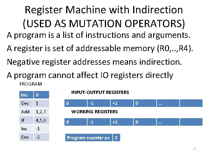
Register Machine with Indirection (USED AS MUTATION OPERATORS) A program is a list of instructions and arguments. A register is set of addressable memory (R 0, . . , R 4). Negative register addresses means indirection. A program cannot affect IO registers directly PROGRAM Inc 0 Dec 1 Add 1, 2, 3 If 4, 5, 6 Inc -1 Dec -2 INPUT-OUTPUT REGISTERS 0 -1 +1 0 … WORKING REGISTERS 0 -1 +1 Program counter pc 2 9

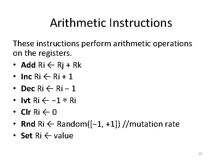
Arithmetic Instructions These instructions perform arithmetic operations on the registers. • Add Ri ← Rj + Rk • Inc Ri ← Ri + 1 • Dec Ri ← Ri − 1 • Ivt Ri ← − 1 ∗ Ri • Clr Ri ← 0 • Rnd Ri ← Random([− 1, +1]) //mutation rate • Set Ri ← value 10

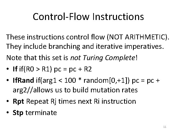
Control-Flow Instructions These instructions control flow (NOT ARITHMETIC). They include branching and iterative imperatives. Note that this set is not Turing Complete! • If if(R 0 > R 1) pc = pc + R 2 • If. Rand if(arg 1 < 100 * random[0, +1]) pc = pc + arg 2//allows us to build mutation rates • Rpt Repeat Rj times next Ri instruction • Stp terminate 11

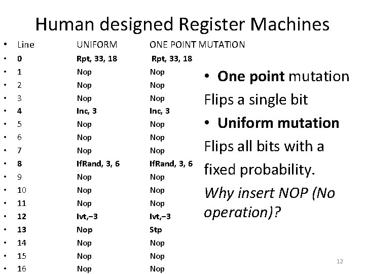
Human designed Register Machines • Line • • • • • 0 1 2 3 4 5 6 7 8 9 10 11 12 13 14 15 16 UNIFORM ONE POINT MUTATION Rpt, 33, 18 Nop Nop Inc, 3 Nop Nop If. Rand, 3, 6 Nop Nop Ivt, − 3 Nop Nop Rpt, 33, 18 Nop Nop Inc, 3 Nop Nop If. Rand, 3, 6 Nop Nop Ivt, − 3 Stp Nop Nop • One point mutation Flips a single bit • Uniform mutation Flips all bits with a fixed probability. Why insert NOP (No operation)? 12

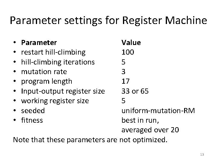
Parameter settings for Register Machine Value 100 5 3 17 33 or 65 5 uniform-mutation-RM best in run, averaged over 20 Note that these parameters are not optimized. • • • Parameter restart hill-climbing iterations mutation rate program length Input-output register size working register size seeded fitness 13

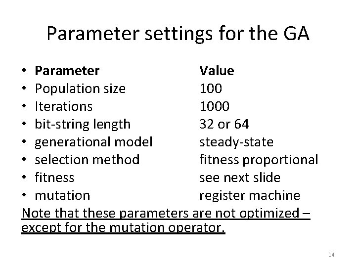
Parameter settings for the GA • Parameter Value • Population size 100 • Iterations 1000 • bit-string length 32 or 64 • generational model steady-state • selection method fitness proportional • fitness see next slide • mutation register machine Note that these parameters are not optimized – except for the mutation operator. 14

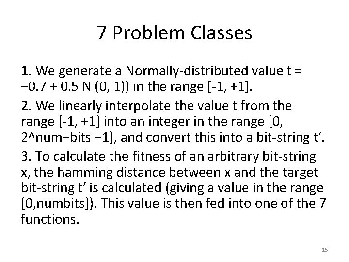
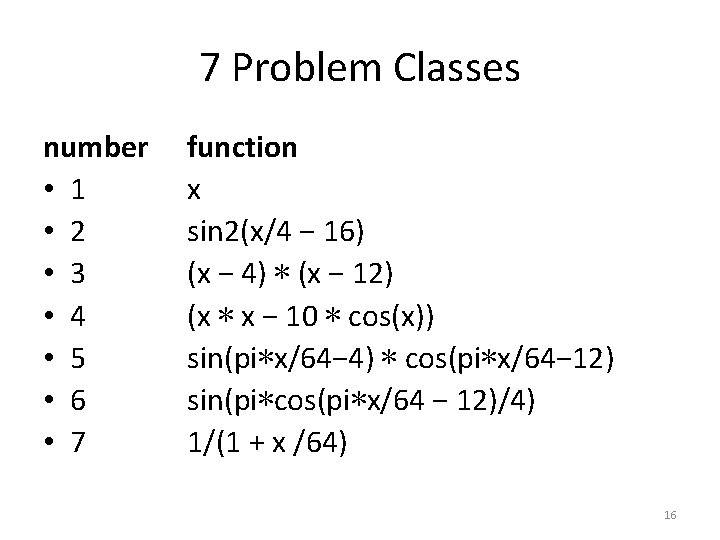
7 Problem Classes 1. We generate a Normally-distributed value t = − 0. 7 + 0. 5 N (0, 1)) in the range [-1, +1]. 2. We linearly interpolate the value t from the range [-1, +1] into an integer in the range [0, 2^num−bits − 1], and convert this into a bit-string t′. 3. To calculate the fitness of an arbitrary bit-string x, the hamming distance between x and the target bit-string t′ is calculated (giving a value in the range [0, numbits]). This value is then fed into one of the 7 functions. 15

7 Problem Classes number • 1 • 2 • 3 • 4 • 5 • 6 • 7 function x sin 2(x/4 − 16) (x − 4) ∗ (x − 12) (x ∗ x − 10 ∗ cos(x)) sin(pi∗x/64− 4) ∗ cos(pi∗x/64− 12) sin(pi∗cos(pi∗x/64 − 12)/4) 1/(1 + x /64) 16

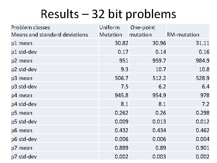
Results – 32 bit problems Problem classes Means and standard deviations p 1 mean p 1 std-dev p 2 mean p 2 std-dev p 3 mean p 3 std-dev p 4 mean p 4 std-dev p 5 mean p 5 std-dev p 6 mean p 6 std-dev p 7 mean p 7 std-dev Uniform One-point Mutation mutation RM-mutation 30. 82 30. 96 31. 11 0. 17 0. 14 0. 16 951 959. 7 984. 9 9. 3 10. 7 10. 8 506. 7 512. 2 528. 9 7. 5 6. 2 6. 4 945. 8 954. 9 978 8. 1 7. 2 0. 26 0. 298 0. 009 0. 013 0. 012 0. 434 0. 462 0. 006 0. 004 0. 889 0. 901 17 0. 002 0. 003 0. 002

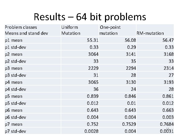
Results – 64 bit problems Problem classes Means and stand dev p 1 mean p 1 std-dev p 2 mean p 2 std-dev p 3 mean p 3 std-dev p 4 mean p 4 std-dev p 5 mean p 5 std-dev p 6 mean p 6 std-dev p 7 mean p 7 std-dev Uniform Mutation One-point mutation 55. 31 0. 33 3064 33 2229 31 3065 36 0. 839 0. 012 0. 643 0. 004 0. 752 0. 0028 RM-mutation 56. 08 56. 47 0. 29 0. 33 3141 3168 35 33 2294 2314 28 27 3130 3193 24 28 0. 846 0. 861 0. 012 0. 643 0. 663 0. 004 0. 003 0. 7529 0. 7684 18 0. 004 0. 0031

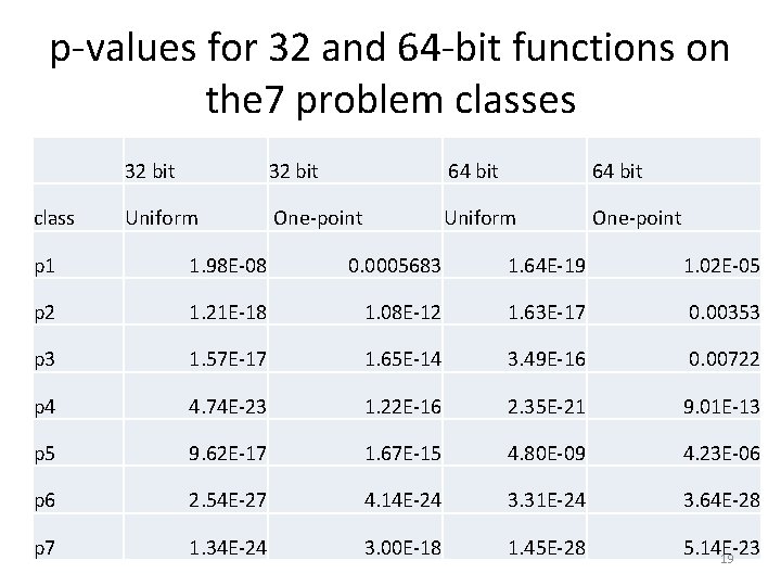
p-values for 32 and 64 -bit functions on the 7 problem classes class 32 bit 64 bit Uniform One-point p 1 1. 98 E-08 0. 0005683 1. 64 E-19 1. 02 E-05 p 2 1. 21 E-18 1. 08 E-12 1. 63 E-17 0. 00353 p 3 1. 57 E-17 1. 65 E-14 3. 49 E-16 0. 00722 p 4 4. 74 E-23 1. 22 E-16 2. 35 E-21 9. 01 E-13 p 5 9. 62 E-17 1. 67 E-15 4. 80 E-09 4. 23 E-06 p 6 2. 54 E-27 4. 14 E-24 3. 31 E-24 3. 64 E-28 p 7 1. 34 E-24 3. 00 E-18 1. 45 E-28 5. 14 E-23 19

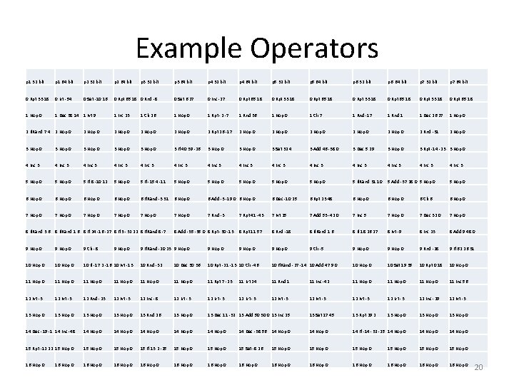
Example Operators p 1 32 bit p 1 64 bit p 2 32 bit p 2 64 bit 0 Rpt 33 18 0 Ivt -54 0 Set -10 16 1 Nop 0 p 3 64 bit p 4 32 bit p 4 64 bit p 5 32 bit p 5 64 bit p 6 32 bit p 6 64 bit p 7 32 bit p 7 64 bit 0 Rpt 65 18 0 Rnd -8 0 Set 6 27 0 Inc -27 0 Rpt 65 18 0 Rpt 33 18 0 Rpt 65 18 1 Dec 38 14 1 Ivt 9 1 Inc 23 1 Clr 26 1 Nop 0 1 Rpt -2 -7 1 Rnd 36 1 Nop 0 1 Clr 7 1 Rnd -17 1 Rnd 1 1 Dec 26 27 1 Nop 0 2 If. Rand 7 4 2 Nop 0 2 Nop 0 2 Rpt 26 -17 2 Nop 0 2 Nop 0 2 Rnd -31 2 Nop 0 3 Nop 0 3 If 40 39 -26 3 Nop 0 3 Set 32 4 3 Add 46 -38 0 3 Dec 5 29 3 Nop 0 3 Rpt -14 -23 3 Nop 0 4 Inc 3 4 Inc 3 4 Inc 3 4 Inc 3 5 Nop 0 5 If 8 -10 12 5 Nop 0 5 If -15 4 -11 5 Nop 0 5 Nop 0 5 If. Rand 31 10 5 Add -37 28 0 5 Nop 0 6 Nop 0 6 If. Rand -3 31 6 Nop 0 6 Add -3 -19 0 6 Nop 0 6 Dec -10 25 6 Rpt 23 48 6 Nop 0 6 Clr 6 6 Nop 0 7 Nop 0 7 Rnd -3 7 Rpt 41 -43 7 Ivt 25 7 Add 53 -42 0 7 Inc 5 7 Nop 0 7 Dec 32 0 7 Nop 0 8 If. Rand 3 6 8 If. Rand 1 6 8 If 24 -16 -27 8 If 3 -32 22 8 If. Rand 8 -7 8 Rpt 11 57 8 Rnd -18 8 If. Rand 1 6 8 If 18 26 27 8 Ivt -9 8 Inc 23 8 Add 9 48 0 9 Nop 0 9 Clr -8 9 Nop 0 9 Clr -5 9 Nop 0 9 Rnd -28 9 If 62 26 31 10 Nop 0 11 Nop 0 8 Add -35 0 8 Rpt -30 -13 4 Inc 3 9 If. Rand -20 23 9 Nop 0 10 If -17 2 -16 10 Ivt -13 10 Rnd -32 10 Dec 30 36 10 Rpt -21 -13 10 Clr -46 10 If. Rand -27 -14 10 Add 47 9 0 10 Nop 0 10 Set 19 35 10 Rpt 0 18 10 Nop 0 11 Nop 0 11 Rpt 7 -23 11 Ivt 24 11 Rnd 1 11 Inc -42 11 Nop 0 11 Inc 56 12 Ivt -3 12 Rnd -23 12 Ivt -3 12 Inc -8 12 Ivt -3 12 Ivt -3 12 Inc -29 12 Ivt -3 13 Nop 0 13 Rnd 26 13 Nop 0 13 Dec 11 -32 13 Add 50 30 0 13 Inc 25 13 Set 17 45 13 Rpt 29 2 13 Nop 0 14 Dec -19 -1 14 Inc -48 14 Nop 0 14 Nop 0 14 Dec -38 56 14 Nop 0 14 If -14 -32 -25 14 Nop 0 15 Rpt -12 22 15 Nop 0 15 If 13 2 -25 15 Nop 0 15 Set -8 26 15 Nop 0 15 Nop 0 16 Nop 0 16 Nop 0 16 Nop 0 16 Nop 0 9 Nop 0 p 3 32 bit 20

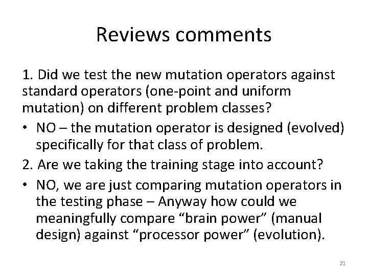
Reviews comments 1. Did we test the new mutation operators against standard operators (one-point and uniform mutation) on different problem classes? • NO – the mutation operator is designed (evolved) specifically for that class of problem. 2. Are we taking the training stage into account? • NO, we are just comparing mutation operators in the testing phase – Anyway how could we meaningfully compare “brain power” (manual design) against “processor power” (evolution). 21

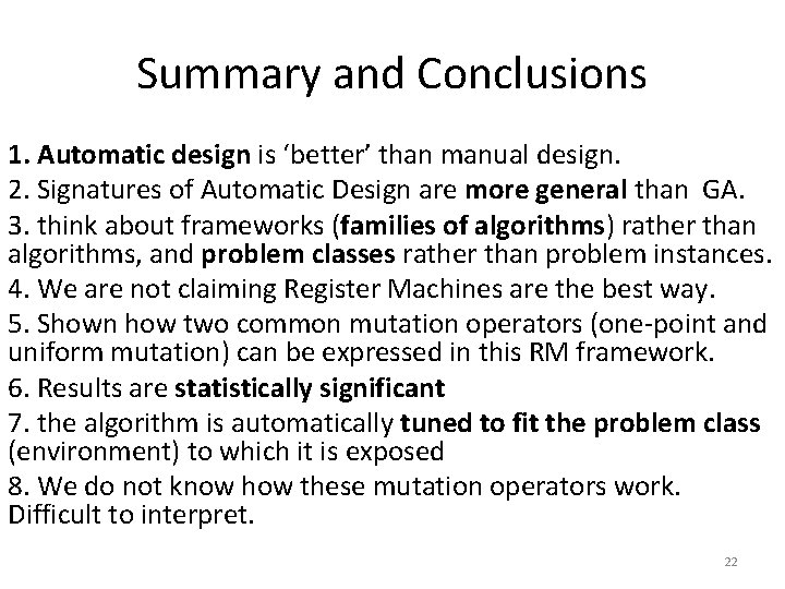
Summary and Conclusions 1. Automatic design is ‘better’ than manual design. 2. Signatures of Automatic Design are more general than GA. 3. think about frameworks (families of algorithms) rather than algorithms, and problem classes rather than problem instances. 4. We are not claiming Register Machines are the best way. 5. Shown how two common mutation operators (one-point and uniform mutation) can be expressed in this RM framework. 6. Results are statistically significant 7. the algorithm is automatically tuned to fit the problem class (environment) to which it is exposed 8. We do not know how these mutation operators work. Difficult to interpret. 22

References • C. Giraud-Carrier and F. Provost. Toward a Justification of Metalearning: Is the No Free Lunch Theorem a Show-stopper? In Proceedings of the ICML-2005 Workshop on Meta-learning, pages 12– 19, 2005. • Jonathan E. Rowe and Michael D. Vose. Unbiased black box search algorithms. In Proceedings of the 13 th annual conference on Genetic and evolutionary computation, GECCO ’ 11, pages 2035– 2042, New. York, NY, USA, 2011. ACM. • J. R. Woodward and J. Swan. Automatically designing selection heuristics. In Proceedings of the 13 th annual conference companion on Genetic and evolutionary computation, pages 583– 590. ACM, 2011. • Edmund K. Burke, Mathew R. Hyde, Graham Kendall, Gabriela Ochoa, Ender Ozcan, and John R. Woodward. Exploring hyperheuristic methodologies with genetic programming. 23

…and Finally • Thank you • Any questions or comments • I hope to see you next year at this workshop. 24