The Aggregate Market For an individual good the

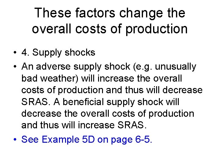
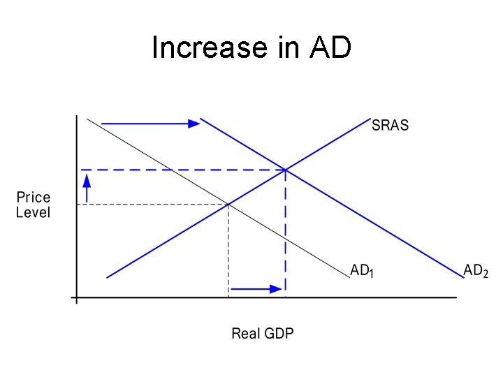
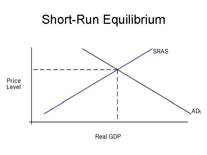
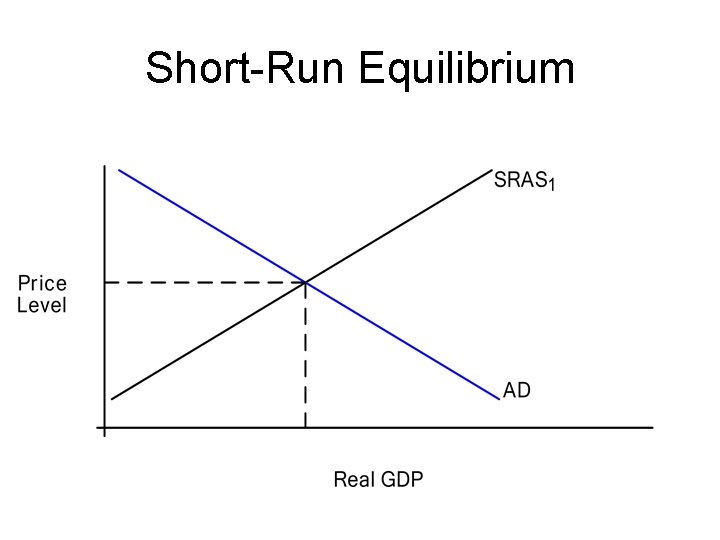
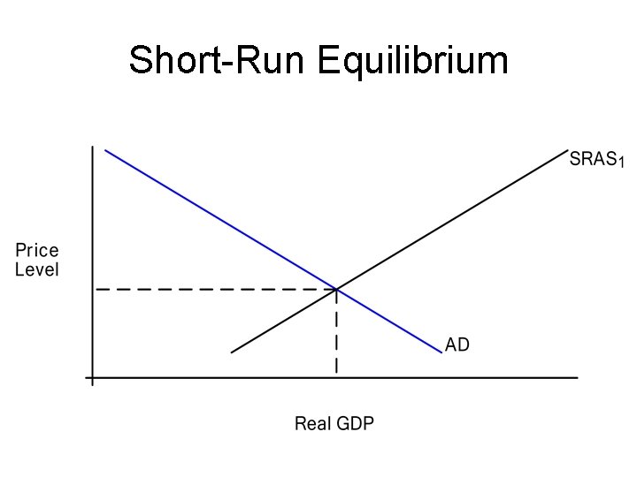
The Aggregate Market • For an individual good, the equilibrium price and quantity are determined by demand supply in the market for that good. • In the overall economy, the price level and the quantity of Real GDP are determined by aggregate demand aggregate supply in the aggregate market.

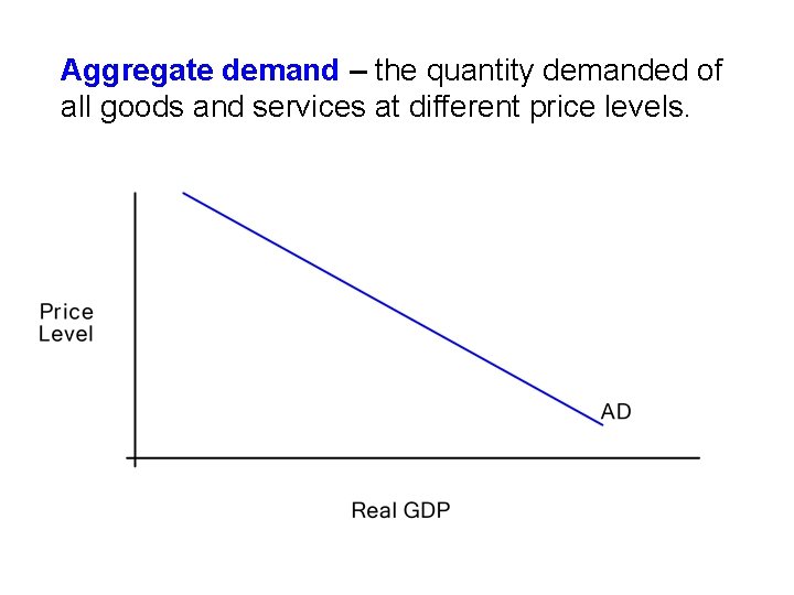
Aggregate demand – the quantity demanded of all goods and services at different price levels.

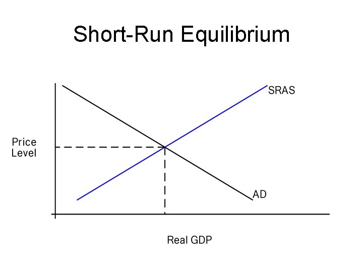
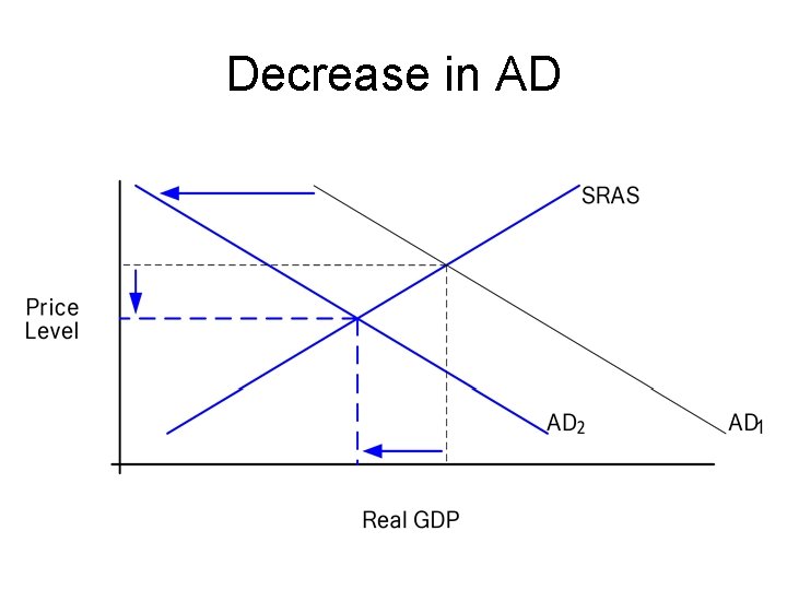
Shifts in the Aggregate Demand Curve • The AD curve shifts in response to changes in Total Expenditures. • An increase in TE will cause an increase in AD. • A decrease in TE will cause a decrease in AD.

Total Expenditures • 1. Consumption • 2. Investment • 3. Government purchases • 4. Net exports

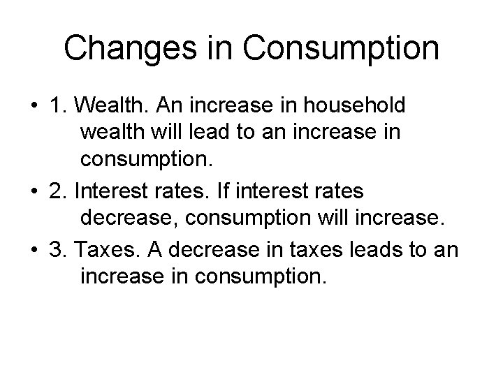
Changes in Consumption • 1. Wealth. An increase in household wealth will lead to an increase in consumption. • 2. Interest rates. If interest rates decrease, consumption will increase. • 3. Taxes. A decrease in taxes leads to an increase in consumption.

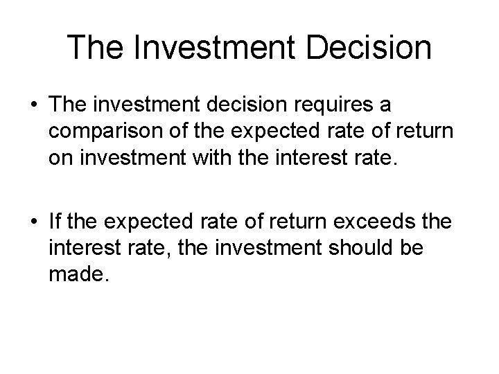
The Investment Decision • The investment decision requires a comparison of the expected rate of return on investment with the interest rate. • If the expected rate of return exceeds the interest rate, the investment should be made.

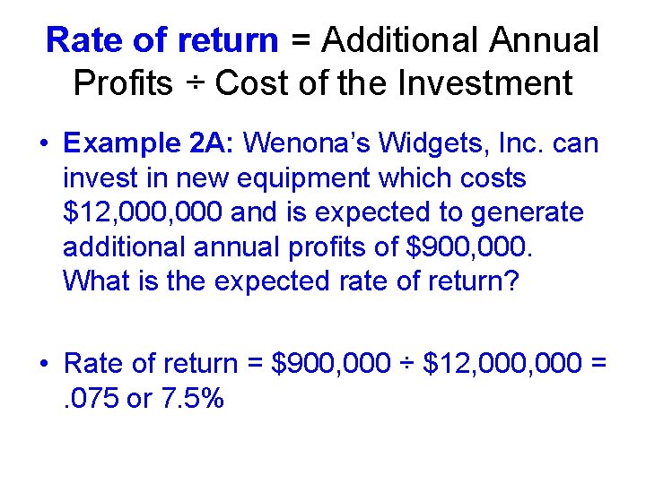
Rate of return = Additional Annual Profits ÷ Cost of the Investment • Example 2 A: Wenona’s Widgets, Inc. can invest in new equipment which costs $12, 000 and is expected to generate additional annual profits of $900, 000. What is the expected rate of return? • Rate of return = $900, 000 ÷ $12, 000 =. 075 or 7. 5%

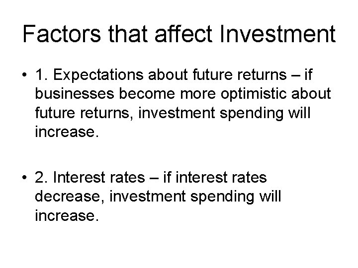
Factors that affect Investment • 1. Expectations about future returns – if businesses become more optimistic about future returns, investment spending will increase. • 2. Interest rates – if interest rates decrease, investment spending will increase.

Government Purchases • The amount of government purchases is determined through the political process. • If the federal, state, or local governments decide to increase spending on goods and services, government purchases will increase.

Net Exports will increase if: • 1. There is an increase in foreign Real GDP. • If U. S. trading partners experience economic growth, they will consume more U. S. exports.

Net Exports will increase if: • 2. The exchange rate for the U. S. dollar depreciates (decreases relative to other currencies). • If the exchange rate for the dollar depreciates, U. S. exports will be cheaper and imports will be more expensive.

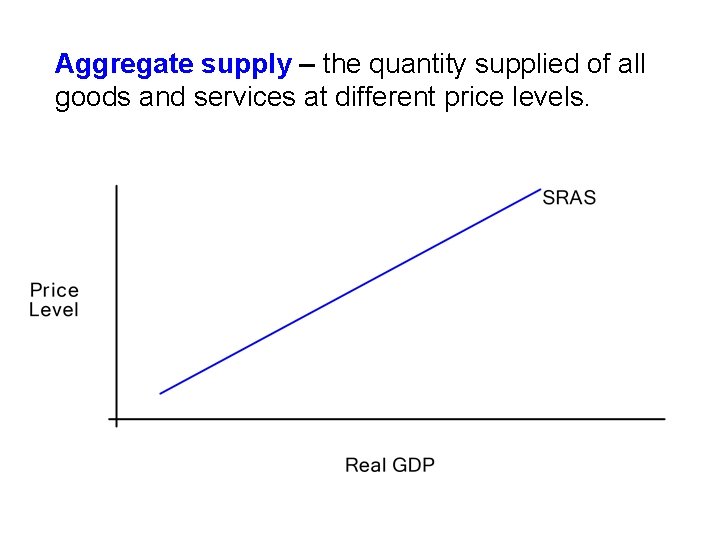
Aggregate supply – the quantity supplied of all goods and services at different price levels.

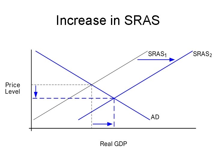
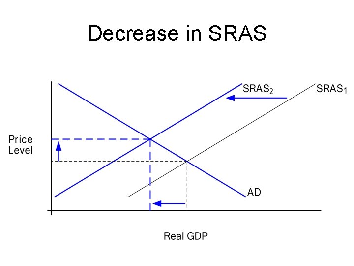
Shifts in the SRAS Curve • The short-run aggregate supply curve shifts in response to changes in the overall costs of production. • An increase in the overall costs of production will cause a decrease in SRAS. • A decrease in the overall costs of production will cause an increase in SRAS.

These factors change the overall costs of production • 1. Wage rates • An increase in wage rates in the economy will increase the overall costs of production and thus will decrease SRAS. A decrease in wage rates will increase SRAS. • See Example 5 A on page 6 -4.

These factors change the overall costs of production • 2. Prices of nonlabor inputs • An increase in the prices of nonlabor inputs (e. g. rent, utilities, insurance, fuel, etc. ) will increase the overall costs of production and thus will decrease SRAS. A decrease in the prices of nonlabor inputs will increase SRAS. • See Example 5 B on page 6 -5.

These factors change the overall costs of production • 3. Productivity • Productivity is measured by the output produced per unit of input. • An increase in productivity will decrease the overall costs of production and thus will increase SRAS. • See Example 5 C on page 6 -5.

These factors change the overall costs of production • 4. Supply shocks • An adverse supply shock (e. g. unusually bad weather) will increase the overall costs of production and thus will decrease SRAS. A beneficial supply shock will decrease the overall costs of production and thus will increase SRAS. • See Example 5 D on page 6 -5.

Short-Run Equilibrium

Increase in AD

Short-Run Equilibrium

Decrease in AD

Short-Run Equilibrium

Increase in SRAS

Short-Run Equilibrium

Decrease in SRAS

SRAS and the Price Level • As labor productivity increases, the SRAS curve shifts to the right. • This should lead to an increase in Real GDP and a decrease in the price level.

SRAS and the Price Level • Real GDP increased by almost 3 -fold between 1978 and 2017. • The CPI increased by about 4 -fold between 1978 and 2017.

SRAS and the Price Level • The price level increased because AD increased faster than SRAS. • AD increased rapidly because the money supply increased rapidly. • See Example 7 on page 6 -8.

SRAS and the Price Level • Increasing SRAS has caused goods to become more affordable. • See Example 8 on page 6 -8.

Why the AD Curve Slopes Downward • 1. The wealth (real balance) effect. • 2. The interest rate effect. • 3. The exchange rate effect.

Why the SRAS Curve Slopes Upward • 1. Sticky-wage effect. • 2. Sticky-price effect. • 3. Misperception effect.