The Academy of Economic Studies Doctoral School of

The Academy of Economic Studies Doctoral School of Finance and Banking Exchange Rate Pass-Through into Inflation in Romania MSc student Ciurilă Nicoleta Coordinator Professor Moisă Altăr Bucharest, July 2006

Dissertation paper outline §The importance of the exchange rate pass-through §The aims of the paper § Empirical studies concerning exchange rate pass-through §The Data §The VAR approach §The single equation approach §Conclusions §References

The importance of exchange rate pass-through Exchange rate pass through - “the percentage change in local currency import prices resulting from a one percent change in the exchange rate between the importing and the exporting countries” (Goldberg and Knetter (1997)) – the change in import prices is passed to some extent into producer and consumer prices Taylor (2000)-importance in the conduct of monetary policy because of its impact on inflation forecasts. Countries that experience high exchange rate pass-through tend to put more emphasis on exchange rate in the conduct of their monetary policyespecially emerging and transition countries. Pass through has an important role in EU acceding countries which will face additional constraints because of ERMII criteria. Edwards(2006)- a high pass-through into nontradable goods prices reduces the effectiveness of the exchange rate, while a high pass through into tradable goods prices will enhance its effectiveness.

The aims of the paper • To quantify the size and speed of the exchange rate pass through into inflation; • To test whether the size of the pass through is dependant on the currency chosen as the base currency; • To determine the variables which account for inflation variability; • To determine whether the size of the pass through has declined in time; • to test if exchange rate volatility influences the size of the pass through; • to check for asymmetries in the exchange rate pass-through.

Empirical studies concerning exchange rate pass -through • • • Single equation method: all studies before 1995, Goldberg and Knetter (1997), Campa and Minguez (2002), Campa, Goldberg and Minguez (2005), Elkayam (2004), Edwards (2006). VAR method and cointegration analysis: Kim (1998), Mc. Carthy (2000), Hahn(2003), Leigh and Rossi(2002), Gueorguiev(2003), Billmeier and Bonato (2002), Coricelli, Jazbec, Masten (2004), Huefner and Schroeder (2002), Arnostova and Hurnik (2004). Structural models – usually developed by central banks – Quartely Projection Models – Gagnon Ihrig (2004).

Adjusting the empirical analysis for the characteristics of the Romanian economy • including a central bank reaction function in the model may prove useless as NBR has only recently adopted the interest rate as operating target • import prices are only available on a quarterly basis, so an analysis using these prices isn’t possible in a model using monthly data • it would be more useful to replace CPI based inflation with the inflation computed using the CORE 1 price index

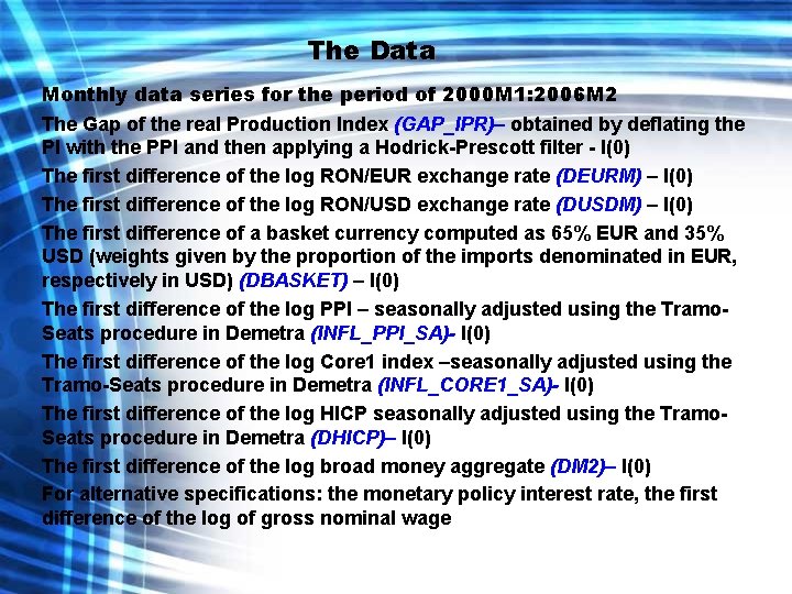
The Data Monthly data series for the period of 2000 M 1: 2006 M 2 The Gap of the real Production Index (GAP_IPR)– obtained by deflating the PI with the PPI and then applying a Hodrick-Prescott filter - I(0) The first difference of the log RON/EUR exchange rate (DEURM) – I(0) The first difference of the log RON/USD exchange rate (DUSDM) – I(0) The first difference of a basket currency computed as 65% EUR and 35% USD (weights given by the proportion of the imports denominated in EUR, respectively in USD) (DBASKET) – I(0) The first difference of the log PPI – seasonally adjusted using the Tramo. Seats procedure in Demetra (INFL_PPI_SA)- I(0) The first difference of the log Core 1 index –seasonally adjusted using the Tramo-Seats procedure in Demetra (INFL_CORE 1_SA)- I(0) The first difference of the log HICP seasonally adjusted using the Tramo. Seats procedure in Demetra (DHICP)– I(0) The first difference of the log broad money aggregate (DM 2)– I(0) For alternative specifications: the monetary policy interest rate, the first difference of the log of gross nominal wage

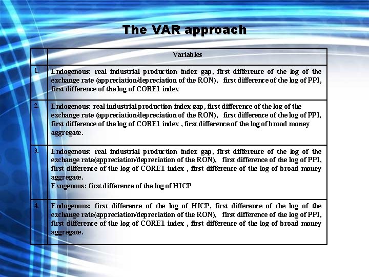
The VAR approach Variables 1. Endogenous: real industrial production index gap, first difference of the log of the exchange rate (appreciation/depreciation of the RON), first difference of the log of PPI, first difference of the log of CORE 1 index 2. Endogenous: real industrial production index gap, first difference of the log of the exchange rate (appreciation/depreciation of the RON), first difference of the log of PPI, first difference of the log of CORE 1 index , first difference of the log of broad money aggregate. 3. Endogenous: real industrial production index gap, first difference of the log of the exchange rate(appreciation/depreciation of the RON), first difference of the log of PPI, first difference of the log of CORE 1 index , first difference of the log of broad money aggregate. Exogenous: first difference of the log of HICP 4. Endogenous: first difference of the log of HICP, first difference of the log of the exchange rate(appreciation/depreciation of the RON), first difference of the log of PPI, first difference of the log of CORE 1 index , first difference of the log of broad money aggregate.

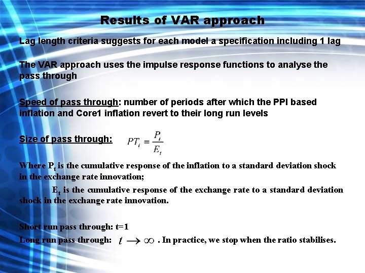
Results of VAR approach Lag length criteria suggests for each model a specification including 1 lag The VAR approach uses the impulse response functions to analyse the pass through Speed of pass through: number of periods after which the PPI based inflation and Core 1 inflation revert to their long run levels Size of pass through: Where Pt is the cumulative response of the inflation to a standard deviation shock in the exchange rate innovation; Et is the cumulative response of the exchange rate to a standard deviation shock in the exchange rate innovation. Short run pass through: t=1 Long run pass through: . In practice, we stop when the ratio stabilises.

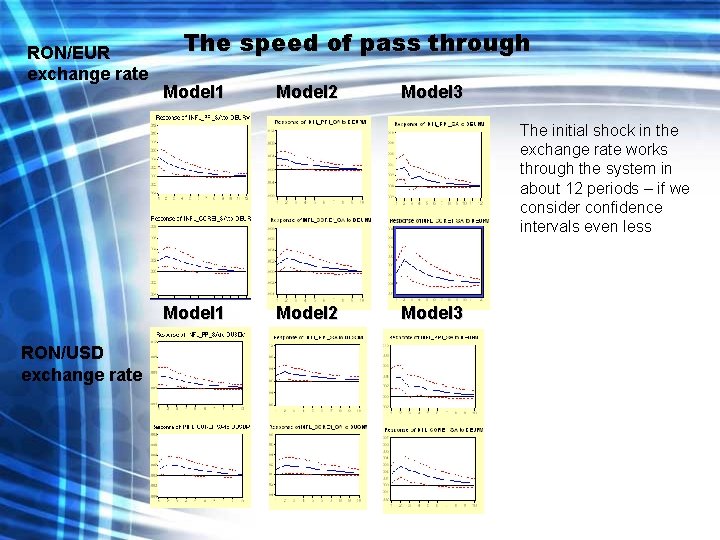
RON/EUR exchange rate The speed of pass through Model 1 Model 2 Model 3 The initial shock in the exchange rate works through the system in about 12 periods – if we consider confidence intervals even less Model 1 RON/USD exchange rate Model 2 Model 3

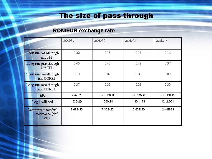
The size of pass through RON/EUR exchange rate Model 1 Model 2 Model 3 Model 4 Short run pass-through into PPI 0. 22 0. 18 0. 17 0. 16 Long run pass-through into PPI 0. 45 0. 40 0. 42 0. 37 Short run pass-through into CORE 1 0. 10 0. 07 0. 06 0. 07 Long run pass-through into CORE 1 0. 37 0. 32 0. 33 0. 30 AIC -24. 32 -29. 96631 -29. 61585 -32. 86004 Log likelihood 919. 89 1090. 88 1101. 171 1212. 961 Determinant residual covariance (dof adj. ) 2. 48 E-16 7. 35 E-20 5. 96 E-20 2. 48 E-21

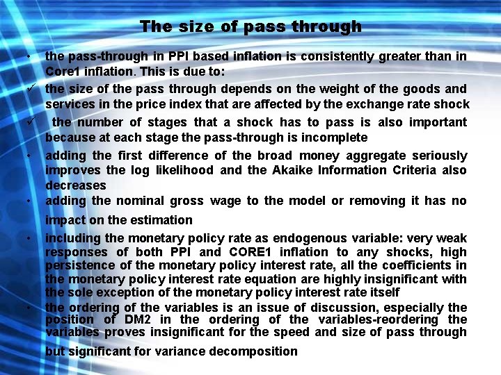
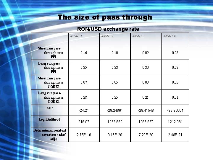
The size of pass through • the pass-through in PPI based inflation is consistently greater than in Core 1 inflation. This is due to: ü the size of the pass through depends on the weight of the goods and services in the price index that are affected by the exchange rate shock ü the number of stages that a shock has to pass is also important because at each stage the pass-through is incomplete • adding the first difference of the broad money aggregate seriously improves the log likelihood and the Akaike Information Criteria also decreases • adding the nominal gross wage to the model or removing it has no • • impact on the estimation including the monetary policy rate as endogenous variable: very weak responses of both PPI and CORE 1 inflation to any shocks, high persistence of the monetary policy interest rate, all the coefficients in the monetary policy interest rate equation are highly insignificant with the sole exception of the monetary policy interest rate itself the ordering of the variables is an issue of discussion, especially the position of DM 2 in the ordering of the variables-reordering the variables proves insignificant for the speed and size of pass through but significant for variance decomposition

The size of pass through RON/USD exchange rate Model 1 Model 2 Model 3 Model 4 Short run passthrough into PPI 0. 16 0. 10 0. 09 0. 08 Long run passthrough into PPI 0. 35 0. 33 0. 30 0. 28 Short run passthrough into CORE 1 0. 07 0. 05 0. 03 Long run passthrough into CORE 1 0. 28 0. 25 0. 21 -24. 21 -29. 24861 -29. 41548 -32. 86004 916. 07 1082. 950 1093. 957 1212. 961 2. 75 E-16 9. 17 E-20 7. 29 E-20 2. 48 E-21 AIC Log likelihood Determinant residual covariance (dof adj. )

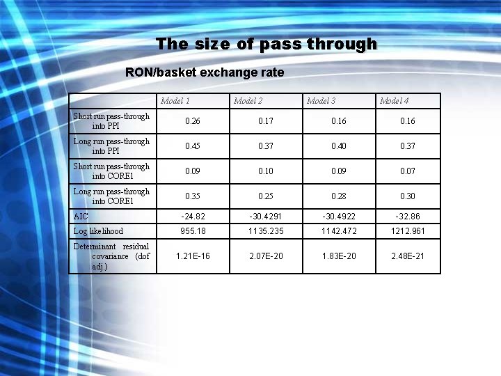
The size of pass through RON/basket exchange rate Model 1 Model 2 Model 3 Model 4 Short run pass-through into PPI 0. 26 0. 17 0. 16 Long run pass-through into PPI 0. 45 0. 37 0. 40 0. 37 Short run pass-through into CORE 1 0. 09 0. 10 0. 09 0. 07 Long run pass-through into CORE 1 0. 35 0. 28 0. 30 AIC -24. 82 -30. 4291 -30. 4922 -32. 86 Log likelihood 955. 18 1135. 235 1142. 472 1212. 961 1. 21 E-16 2. 07 E-20 1. 83 E-20 2. 48 E-21 Determinant residual covariance (dof adj. )

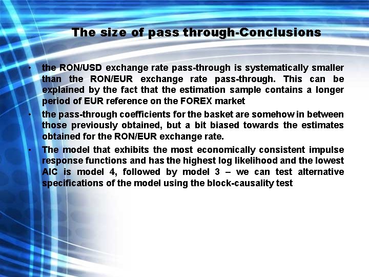
The size of pass through-Conclusions • • • the RON/USD exchange rate pass-through is systematically smaller than the RON/EUR exchange rate pass-through. This can be explained by the fact that the estimation sample contains a longer period of EUR reference on the FOREX market the pass-through coefficients for the basket are somehow in between those previously obtained, but a bit biased towards the estimates obtained for the RON/EUR exchange rate. The model that exhibits the most economically consistent impulse response functions and has the highest log likelihood and the lowest AIC is model 4, followed by model 3 – we can test alternative specifications of the model using the block-causality test

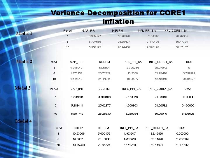
Variance Decomposition for CORE 1 inflation Period Model 1 Model 2 Model 3 Period GAP_IPR DEURM INFL_PPI_SA INFL_CORE 1_SA 1 8. 369197 10. 48878 2. 64847 78. 49355 5 5. 797656 25. 88497 9. 140125 59. 17724 10 5. 558193 26. 94406 9. 326178 58. 17157 GAP_IPR DEURM INFL_PPI_SA INFL_CORE 1_SA DM 2 1 1. 245019 6. 05501 3. 720254 88. 97972 0 5 1. 376158 20. 72329 10. 2058 63. 93476 3. 759999 10 1. 546918 21. 14246 10. 86377 62. 55058 3. 896274 Period GAP_IPR DEURM INFL_PPI_SA INFL_CORE 1_SA DM 2 1 1. 541631 4. 464166 2. 154076 91. 84013 0. 000000 5 5. 283411 25. 02377 4. 900803 58. 29532 6. 496696 10 6. 894712 25. 25839 5. 269784 55. 98049 6. 596625 Model 4 Period DHICP DEURM INFL_PPI_SA INFL_CORE 1_SA DM 2 1 10. 63268 5. 409175 1. 493547 82. 46460 0. 000000 5 19. 39071 20. 13060 4. 927478 53. 31920 2. 232009 10 19. 75258 20. 65724 5. 171728 52. 11691 2. 301542

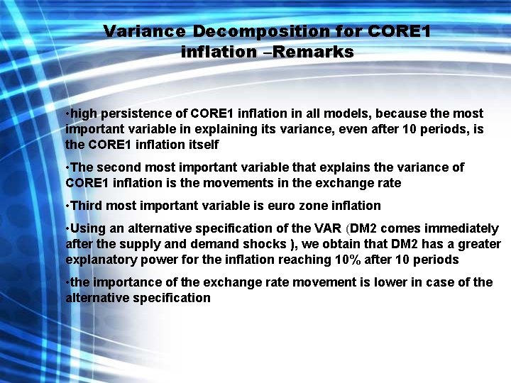
Variance Decomposition for CORE 1 inflation –Remarks • high persistence of CORE 1 inflation in all models, because the most important variable in explaining its variance, even after 10 periods, is the CORE 1 inflation itself • The second most important variable that explains the variance of CORE 1 inflation is the movements in the exchange rate • Third most important variable is euro zone inflation • Using an alternative specification of the VAR (DM 2 comes immediately after the supply and demand shocks ), we obtain that DM 2 has a greater explanatory power for the inflation reaching 10% after 10 periods • the importance of the exchange rate movement is lower in case of the alternative specification

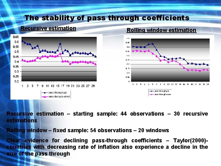
The stability of pass through coefficients Recursive estimation Rolling window estimation Recursive estimation – starting sample: 44 observations – 30 recursive estimations Rolling window – fixed sample: 54 observations – 20 windows Clear evidence for declining pass-through coefficients – Taylor(2000)countries with decreasing rate of inflation also experience a decline in the size of the pass through

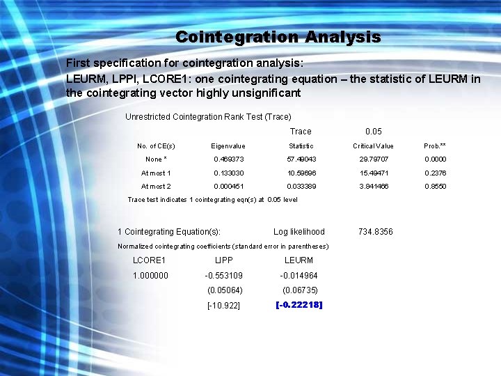
Cointegration Analysis First specification for cointegration analysis: LEURM, LPPI, LCORE 1: one cointegrating equation – the statistic of LEURM in the cointegrating vector highly unsignificant Unrestricted Cointegration Rank Test (Trace) Trace 0. 05 No. of CE(s) Eigenvalue Statistic Critical Value Prob. ** None * 0. 469373 57. 49043 29. 79707 0. 0000 At most 1 0. 133030 10. 59696 15. 49471 0. 2376 At most 2 0. 000451 0. 033389 3. 841466 0. 8550 Trace test indicates 1 cointegrating eqn(s) at 0. 05 level 1 Cointegrating Equation(s): Log likelihood Normalized cointegrating coefficients (standard error in parentheses) LCORE 1 LIPP LEURM 1. 000000 -0. 553109 -0. 014964 (0. 05064) (0. 06735) [-10. 922] [-0. 22218] 734. 8356

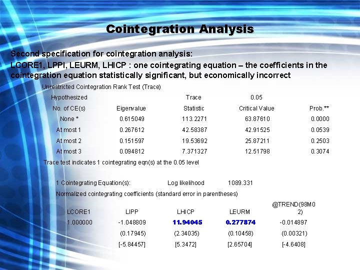
Cointegration Analysis Second specification for cointegration analysis: LCORE 1, LPPI, LEURM, LHICP : one cointegrating equation – the coefficients in the cointegration equation statistically significant, but economically incorrect Unrestricted Cointegration Rank Test (Trace) Hypothesized Trace 0. 05 No. of CE(s) Eigenvalue Statistic Critical Value Prob. ** None * 0. 615049 113. 2271 63. 87610 0. 0000 At most 1 0. 267612 42. 58387 42. 91525 0. 0539 At most 2 0. 151597 19. 53692 25. 87211 0. 2503 At most 3 0. 094812 7. 371327 12. 51798 0. 3074 Trace test indicates 1 cointegrating eqn(s) at the 0. 05 level 1 Cointegrating Equation(s): Log likelihood 1089. 331 Normalized cointegrating coefficients (standard error in parentheses) LCORE 1 LIPP LHICP LEURM @TREND(98 M 0 2) 1. 000000 -1. 048809 11. 94045 0. 277874 -0. 014897 (0. 17945) (2. 34035) (0. 10458) (0. 00321) [-5. 84457] [5. 3472] [2. 65704] [-4. 6408]

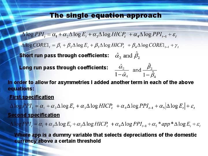
The single equation approach Short run pass through coefficients: Long run pass through coefficients: In order to allow for asymmetries I added another term in each of the above equations: First specification Second specification Where app is a dummy variable that selects depreciations of the domestic currency above a certain threshold

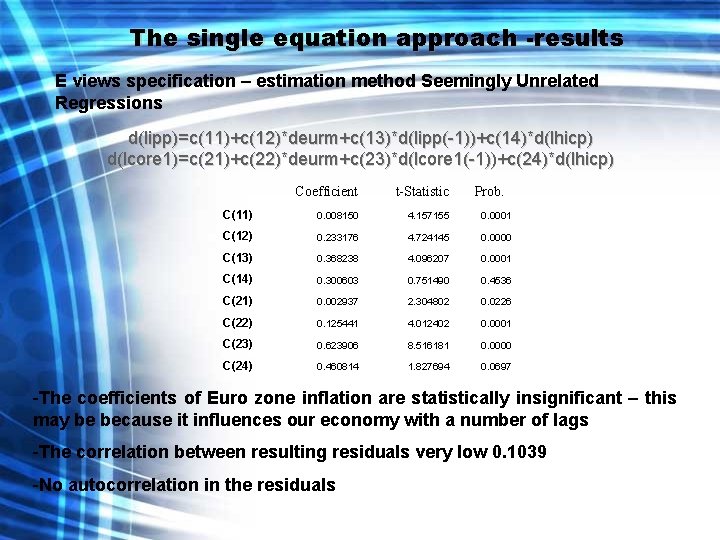
The single equation approach -results E views specification – estimation method Seemingly Unrelated Regressions d(lipp)=c(11)+c(12)*deurm+c(13)*d(lipp(-1))+c(14)*d(lhicp) d(lcore 1)=c(21)+c(22)*deurm+c(23)*d(lcore 1(-1))+c(24)*d(lhicp) Coefficient t-Statistic Prob. C(11) 0. 008150 4. 157155 0. 0001 C(12) 0. 233176 4. 724145 0. 0000 C(13) 0. 368238 4. 096207 0. 0001 C(14) 0. 300603 0. 751490 0. 4536 C(21) 0. 002937 2. 304802 0. 0226 C(22) 0. 125441 4. 012402 0. 0001 C(23) 0. 623906 8. 516181 0. 0000 C(24) 0. 460814 1. 827694 0. 0697 -The coefficients of Euro zone inflation are statistically insignificant – this may be because it influences our economy with a number of lags -The correlation between resulting residuals very low 0. 1039 -No autocorrelation in the residuals

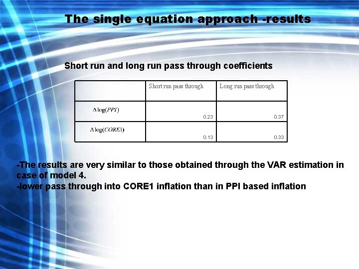
The single equation approach -results Short run and long run pass through coefficients Short run pass through Long run pass through 0. 23 0. 37 0. 13 0. 33 -The results are very similar to those obtained through the VAR estimation in case of model 4. -lower pass through into CORE 1 inflation than in PPI based inflation

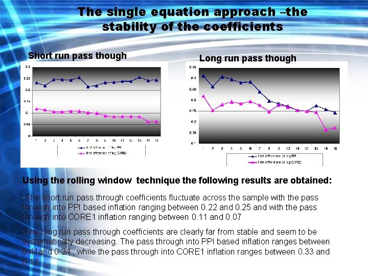
The single equation approach –the stability of the coefficients Short run pass though Long run pass though Using the rolling window technique the following results are obtained: -The short run pass through coefficients fluctuate across the sample with the pass through into PPI based inflation ranging between 0. 22 and 0. 25 and with the pass through into CORE 1 inflation ranging between 0. 11 and 0. 07 -The long run pass through coefficients are clearly far from stable and seem to be systematically decreasing. The pass through into PPI based inflation ranges between 0. 41 and 0. 24 , while the pass through into CORE 1 inflation ranges between 0. 33 and 0. 17

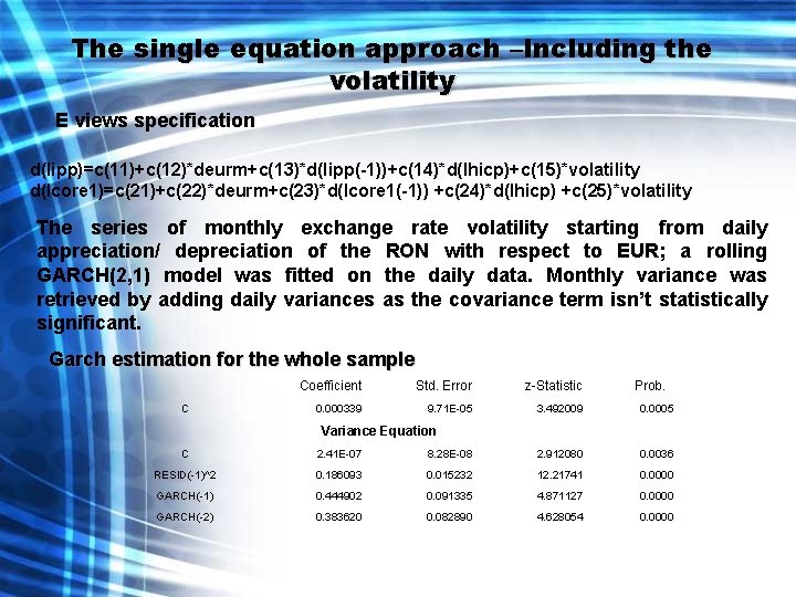
The single equation approach –Including the volatility E views specification d(lipp)=c(11)+c(12)*deurm+c(13)*d(lipp(-1))+c(14)*d(lhicp)+c(15)*volatility d(lcore 1)=c(21)+c(22)*deurm+c(23)*d(lcore 1(-1)) +c(24)*d(lhicp) +c(25)*volatility The series of monthly exchange rate volatility starting from daily appreciation/ depreciation of the RON with respect to EUR; a rolling GARCH(2, 1) model was fitted on the daily data. Monthly variance was retrieved by adding daily variances as the covariance term isn’t statistically significant. Garch estimation for the whole sample C Coefficient Std. Error z-Statistic Prob. 0. 000339 9. 71 E-05 3. 492009 0. 0005 Variance Equation C 2. 41 E-07 8. 28 E-08 2. 912080 0. 0036 RESID(-1)^2 0. 186093 0. 015232 12. 21741 0. 0000 GARCH(-1) 0. 444902 0. 091335 4. 871127 0. 0000 GARCH(-2) 0. 383620 0. 082890 4. 628054 0. 0000

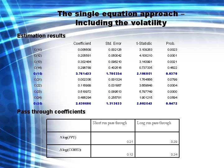
The single equation approach – Including the volatility Estimation results Coefficient Std. Error t-Statistic Prob. C(11) 0. 006609 0. 002126 3. 109263 0. 0023 C(12) 0. 205581 0. 050042 4. 108210 0. 0001 C(13) 0. 302484 0. 096210 3. 143991 0. 0021 C(14) 0. 296789 0. 402516 0. 737335 0. 4622 C(15) 3. 761433 1. 785334 2. 106851 0. 0370 C(21) 0. 002336 0. 001324 1. 764566 0. 0799 C(22) 0. 116989 0. 031967 3. 659648 0. 0004 C(23) 0. 518972 0. 089513 5. 797749 0. 0000 C(24) 0. 486294 0. 255781 1. 901215 0. 0594 C(25) 2. 630606 1. 313633 2. 002543 0. 0472 Pass through coefficients Short run pass through Long run pass through 0. 21 0. 29 0. 12 0. 24

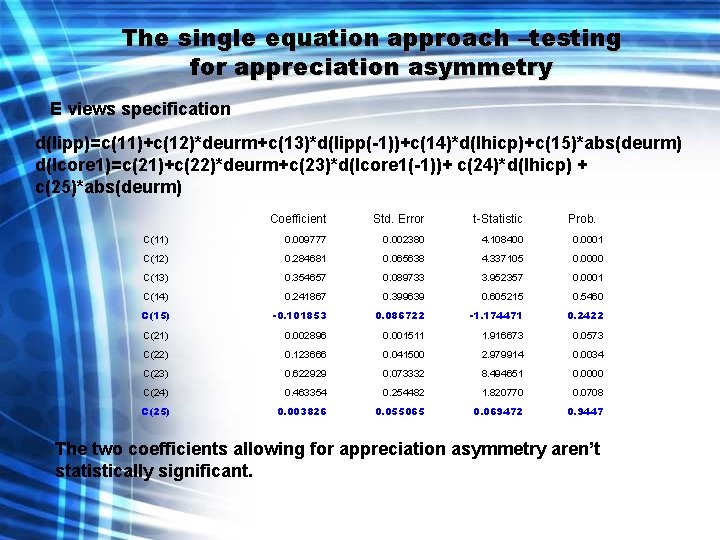
The single equation approach –testing for appreciation asymmetry E views specification d(lipp)=c(11)+c(12)*deurm+c(13)*d(lipp(-1))+c(14)*d(lhicp)+c(15)*abs(deurm) d(lcore 1)=c(21)+c(22)*deurm+c(23)*d(lcore 1(-1))+ c(24)*d(lhicp) + c(25)*abs(deurm) Coefficient Std. Error t-Statistic Prob. C(11) 0. 009777 0. 002380 4. 108400 0. 0001 C(12) 0. 284681 0. 065638 4. 337105 0. 0000 C(13) 0. 354657 0. 089733 3. 952357 0. 0001 C(14) 0. 241867 0. 399639 0. 605215 0. 5460 C(15) -0. 101853 0. 086722 -1. 174471 0. 2422 C(21) 0. 002896 0. 001511 1. 916673 0. 0573 C(22) 0. 123666 0. 041500 2. 979914 0. 0034 C(23) 0. 622929 0. 073332 8. 494651 0. 0000 C(24) 0. 463354 0. 254482 1. 820770 0. 0708 C(25) 0. 003826 0. 055065 0. 069472 0. 9447 The two coefficients allowing for appreciation asymmetry aren’t statistically significant.

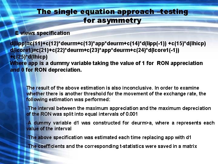
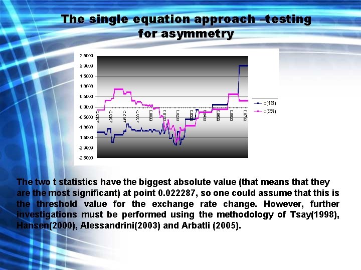
The single equation approach –testing for asymmetry E views specification d(lipp)=c(11)+c(12)*deurm+c(13)*app*deurm+c(14)*d(lipp(-1)) +c(15)*d(lhicp) d(lcore 1)=c(21)+c(22)*deurm+c(23)*app*deurm+c(24)*d(lcore 1(-1)) +c(25)*d(lhicp) Where app is a dummy variable taking the value of 1 for RON appreciation and 0 for RON depreciation. The result of the above estimation is also inconclusive. In order to examine whethere is another threshold for the movement of the exchange rate, the following estimation was performed: -The interval between the maximum appreciation and the maximum depreciation of the RON was split into equal intervals of 0. 001 -A dummy variable d 1 was constructed for deurm>a, where a represents each value of the interval -The above specification was estimated each time replacing app with d 1 -The coefficients and the corresponding t-statistics were saved in a matrix

The single equation approach –testing for asymmetry The two t statistics have the biggest absolute value (that means that they are the most significant) at point 0. 022287, so one could assume that this is the threshold value for the exchange rate change. However, further investigations must be performed using the methodology of Tsay(1998), Hansen(2000), Alessandrini(2003) and Arbatli (2005).

Conclusions • The speed of pass-through: an initial shock in the exchange rate movement completely works through the economy and is passed into producer and consumer prices in 12 months • The size of the pass through varies across the models and across the exchange rates used. The RON/EUR exchange rate pass through into producer prices varies between 0. 37 and 0. 45 depending on the VAR model, while the pass through into consumer prices varies between 0. 30 and 0. 37. • The RON/USD exchange rate pass-through is consistently lower than the RON/EUR, ranging between 0. 28 and 0. 35 for producer prices, and between 0. 21 and 0. 28 for consumer prices • The basket exchange rate pass-through coefficients are for each model found to be between the coefficient of the RON/EUR pass-through and the RON/USD passthrough • Variance decomposition: The percent of the variance explained by different variables varies across models and for model 4 it also varies across alternative orderings of the variables. It is clear however, that the determinants of inflation are the following: inflation itself (78%-90%), the exchange rate movements(21%-27%), HICP inflation (19%) and the variation of the broad monetary aggregate (2%-10%).

Conclusions • • • Using both recursive and the rolling window estimation sufficiently clear evidence was found that the pass through has declined gradually The results of the single equation approach are consistent with the ones obtained through the VAR method: the long run pass through into producer prices is equal to 0. 37 while the long run pass through into consumer prices is equal to 0. 30 The pass through coefficients computed using the single equation approach were also checked for stability using the rolling window approach – the conclusion is the same: pass through in Romania seems to have decreased in the last period. Taking into account exchange rate volatility proved in statistically significant in both equations and changes the pass through coefficients: The long run pass through into producer prices becomes equal to 0. 29 while the long run pass through into consumer prices changes to 0. 24. Including the appreciation of the exchange rate as a distinct explanatory variable in both equations made no difference - the coefficients are not significant - there probably is no asymmetry around the zero value of the exchange rate change. The investigation for a non-zero threshold of the exchange rate change showed as marginally significant a 0. 022287 depreciation as a threshold value

References Amato, J. , Filardo, A. , Galati, G. , von Peter, G. , Zhu, F. (2005): “Research on exchange rates and monetary policy: an overview”, BIS Working paper no. 179 Arbatli, E. (2003): “Exchange Rate Pass Through in Turkey: Looking for Asymmetries”, Central Bank Review, vol. 3, issue 2, pages 85 -124 Brooks, C. (2002) : Introductory Econometrics for Finance , Cambridge University Press Billmeier, A. , Bonato, L. (2002): “Exchange Rate Pass-Through and Monetary Policy in Croatia”, IMF Working Paper, 109/2002 Caner, M. , Hansen, B. (2004): “Instrumental Variable Estimation of a Threshold Model”, Econometric Theory, 20, 813– 843 Coricelli, F. , Jazbec B. , Masten I. (2004) „Exchange Rate Pass-Through in Acceding Countries”, European University Institute Working Paper no. 2004/16 Choudhri E. U. , Faruqee H. , and Hakura D. (2002): “Explaining the Exchange Rate Pass-Through in Different Prices”, IMF Working Paper, 224/2002 Campa, J. M, Gonzalez Minguez, J. M. (2002): “Differences in Exchange Rate Pass-Through in the Euro Area”, IESE Working Paper No. D/479 Christiano, L. , Eichenbaum, M. , Evans, C. (1996) „Sticky Price and Limited Participation Models of Money: A Comparison”, NBER Working Paper no. 5804 Campa, J. M, Goldberg, L. , Gonzalez Minguez , J. M. (2005): „Exchange-Rate Pass-Through To Import Prices In The Euro Area”, NBER Working Paper no. 11632 Edwards, S. (2006): “The Relationship Between Exchange Rates And Inflation Targeting Revisited”, NBER Working Paper no. 12163 Enders, W. (2004): „Applied Time Series Econometrics”, John Wiley & Sons

• Engle, C. , Devereux M. (2002): ”Exchange Rate Pass-Through, Exchange Rate Volatility, and Exchange Rate Disconnect”, NBER working Paper no. 9568 • Gagnon, J. , Ihring, G. (2002): “Monetary Policy and Exchange Rate Pass-Through”, Board of Governors of the Federal Reserve System, International Finance Discussion Paper No. 2001/704. • Goldberg, P. , Knetter, M (1997): “Goods Prices and Exchange Rates: What have we learned? ”, NBER Working Paper no. 5862 • Gueorguiev, N. (2003): “Exchange rate pass through in Romania”, IMF Working Paper, 130/2003 • Hahn, E. (2003): “Pass Through of External Shocks to Euro Area Inflation”, ECB Working Paper, no. 243 • Hufner, F. P, Schroder, M. (2002): “Exchange Rate Pass Through to Consumer Prices: A European Perspective”, Centre for European Economic Research Discussion Paper no. 02 -20 • Leigh, D. , Rossi M. (2002): “Exchange Rate Pass-Through in Turkey”, IMF Working Paper no. 2002/204 • Mc. Carthy, J. (2000): ”Pass-Through of Exchange Rates and Import Prices to Domestic Inflation in Some Industrialized Economies”, Federal Reserve Bank of New York Working Paper • Rowland, P. (2003): “Exchange Rate Pass-Through to Domestic Prices: The Case of Colombia ”Banco de la Republica de Colombia • Sarno, L. , Taylor, M. (2002): “The Economics of Exchange Rates”, Cambridge University Press • Sekine, T. (2006): “Time-varying exchange rate pass-through: experiences of some industrial countries”, BIS Working Paper no 202

• Taylor, J. B. (2000): “Low Inflation, Pass-Through, and the Pricing Power of Firms” European Economic Review vol. 44, issue 7, pages 1389 -1408 • Tsay, R (1998): “Testing and Modeling Multivariate Threshold Models”, Journal of the American Statistical Association , 94, 1188 -1202. • Warne, A (1993) “A Common Trends Model: Identification, Estimation and Inference”, Seminar Paper No. 555, IIES, Stockholm University