The ABCs of Filter Factors aka Selectivity Joe

The ABCs of Filter Factors (aka Selectivity) Joe Geller JPMorgan Chase Session Code: E 12 Wednesday, November 16 th, 2016 14: 30 | Platform: Cross Platform 1

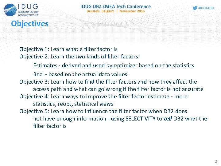
Objectives Objective 1: Learn what a filter factor is Objective 2: Learn the two kinds of filter factors: Estimates - derived and used by optimizer based on the statistics Real - based on the actual data values. Objective 3: Learn how to find the filter factors and how they affect the access path and what can go wrong if the filter factor is not accurate Objective 4: Learn ways to improve the filter factor estimate - more statistics, reopt, statistical views Objective 5: Learn how to influence the filter factor when DB 2 does not have enough information - using SELECTIVITY to tell DB 2 what the filter factor is 2

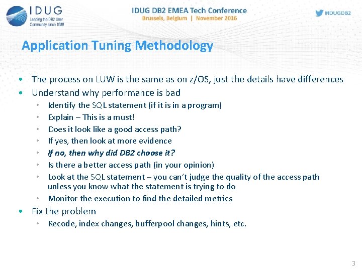
3 Application Tuning Methodology • The process on LUW is the same as on z/OS, just the details have differences • Understand why performance is bad Identify the SQL statement (if it is in a program) Explain – This is a must! Does it look like a good access path? If yes, then look at more evidence If no, then why did DB 2 choose it? Is there a better access path (in your opinion) Look at the SQL statement – you can’t judge the quality of the access path unless you know what the statement is trying to do • Monitor the execution to find the detailed metrics • • Fix the problem • Recode, index changes, bufferpool changes, hints, etc. 3

4 Is it a Good or Bad Access Path? • Understand the different kinds of access path • Understand which are good and which are bad – under what circumstances and conditions • Statistics – what exists? What are the cardinalities of the table, columns and indexes? • Indexes – what are the keys and what are the statistics • Filter Factors 4

Filter Factors (abbreviated FF) • What does “filter” mean? • Remove some items • Air filter – remove dust and other particles • Pool filter • Coffee filter – remove the coffee grinds • What is DB 2 filtering? • Rows 5

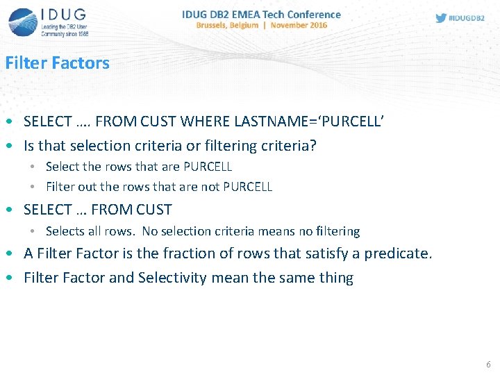
Filter Factors • SELECT …. FROM CUST WHERE LASTNAME=‘PURCELL’ • Is that selection criteria or filtering criteria? • Select the rows that are PURCELL • Filter out the rows that are not PURCELL • SELECT … FROM CUST • Selects all rows. No selection criteria means no filtering • A Filter Factor is the fraction of rows that satisfy a predicate. • Filter Factor and Selectivity mean the same thing 6

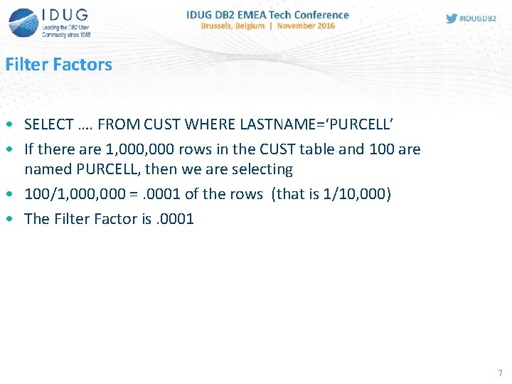
Filter Factors • SELECT …. FROM CUST WHERE LASTNAME=‘PURCELL’ • If there are 1, 000 rows in the CUST table and 100 are named PURCELL, then we are selecting • 100/1, 000 =. 0001 of the rows (that is 1/10, 000) • The Filter Factor is. 0001 7

Filter Factors • Backwards wording? • Selectivity is a better word • Both are used • • Documentation uses both Visual Explain in Data Studio use filter factor Visual Explain in the old Command Editor uses Selectivity db 2 exfmt (LUW) uses filter factor • Why do we care about filter factors? • We care because DB 2 cares (that’s how Terry Purcell would answer that question) 8

Filter Factors • Guideline: • Filter more, earlier. Fewer rows will be left for later steps. • Particularly important to understanding DB 2’s choice of join method and join order. 9

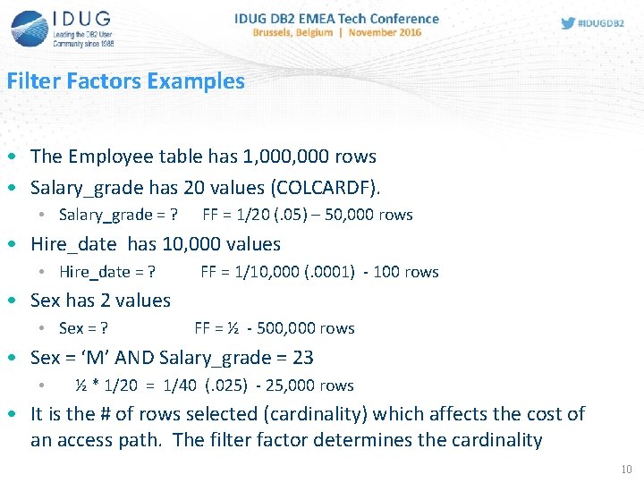
Filter Factors Examples • The Employee table has 1, 000 rows • Salary_grade has 20 values (COLCARDF). • Salary_grade = ? FF = 1/20 (. 05) – 50, 000 rows • Hire_date has 10, 000 values • Hire_date = ? FF = 1/10, 000 (. 0001) - 100 rows • Sex has 2 values • Sex = ? FF = ½ - 500, 000 rows • Sex = ‘M’ AND Salary_grade = 23 • ½ * 1/20 = 1/40 (. 025) - 25, 000 rows • It is the # of rows selected (cardinality) which affects the cost of an access path. The filter factor determines the cardinality 10

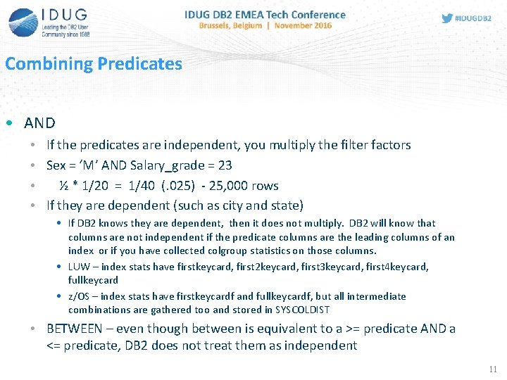
Combining Predicates • AND • If the predicates are independent, you multiply the filter factors • Sex = ‘M’ AND Salary_grade = 23 • ½ * 1/20 = 1/40 (. 025) - 25, 000 rows • If they are dependent (such as city and state) • If DB 2 knows they are dependent, then it does not multiply. DB 2 will know that columns are not independent if the predicate columns are the leading columns of an index or if you have collected colgroup statistics on those columns. • LUW – index stats have firstkeycard, first 2 keycard, first 3 keycard, first 4 keycard, fullkeycard • z/OS – index stats have firstkeycardf and fullkeycardf, but all intermediate combinations are gathered too and stored in SYSCOLDIST • BETWEEN – even though between is equivalent to a >= predicate AND a <= predicate, DB 2 does not treat them as independent 11

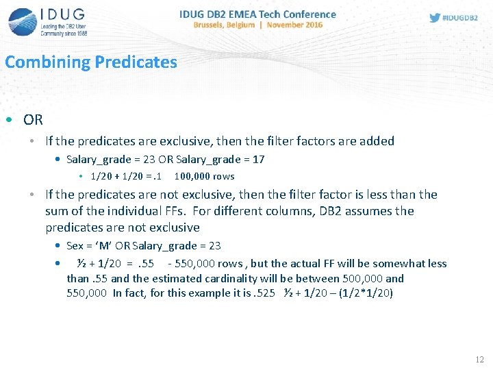
Combining Predicates • OR • If the predicates are exclusive, then the filter factors are added • Salary_grade = 23 OR Salary_grade = 17 • 1/20 + 1/20 =. 1 100, 000 rows • If the predicates are not exclusive, then the filter factor is less than the sum of the individual FFs. For different columns, DB 2 assumes the predicates are not exclusive • Sex = ‘M’ OR Salary_grade = 23 • ½ + 1/20 =. 55 - 550, 000 rows , but the actual FF will be somewhat less than. 55 and the estimated cardinality will be between 500, 000 and 550, 000 In fact, for this example it is. 525 ½ + 1/20 – (1/2*1/20) 12

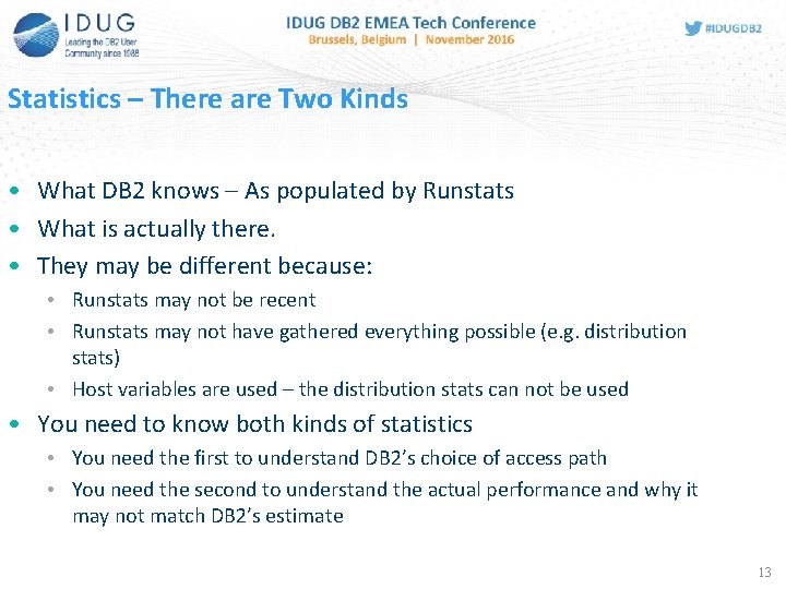
Statistics – There are Two Kinds • What DB 2 knows – As populated by Runstats • What is actually there. • They may be different because: • Runstats may not be recent • Runstats may not have gathered everything possible (e. g. distribution stats) • Host variables are used – the distribution stats can not be used • You need to know both kinds of statistics • You need the first to understand DB 2’s choice of access path • You need the second to understand the actual performance and why it may not match DB 2’s estimate 13

Filter factors – There are Two Kinds • Estimates - based on the statistics in the catalog • Real - based on the actual data values and the values of any host variables at run time • Which kind was the example (LASTNAME=‘PURCELL’) we just looked at? • Real – I told you how many rows there were 14

Statistics – How Do You Know What They Are? • Actual statistics – you have to write queries to find out • Catalog statistics – 2 ways: • Look in the catalog (with SQL or with a tool): • SYSTABLES (CARDF) • SYSCOLUMNS (COLCARDF) • SYSINDEXES (FIRSTKEYCARDF, FULLKEYCARDF) • Filter Factors – the manuals describe the rules and formulas. You can then calculate the filter factor. • Visual Explain • The big advantage of VE is not the picture. If you understand access paths, you can visualize the access path from the Plan_Table (z/OS) - with practice. • The big advantage is that it gathers all the info – index columns, cardinality, filter factors. 15

Filter Factors – How Do You Know What They Are? • Actual filter factors – you have to write queries to find out • DB 2’s estimate – 2 ways: • Manually - you can calculate the filter factor using the statistics in the catalog. • Visual Explain • Gives you the filter factors for each predicate. 16

Calculating Filter Factors • Equal (=) – simple – if there are n values, the FF = 1/n • Range Defaults (no column stats) • >, < etc. – FF = 1/3 • BETWEEN – FF = 1/10 • Range Defaults (with COLCARDF) • Depends on the value of colcardf • >= 1, 000 3/10, 000 • >= 100, 000 1/1000 • Range with Literal • Interpolation 17

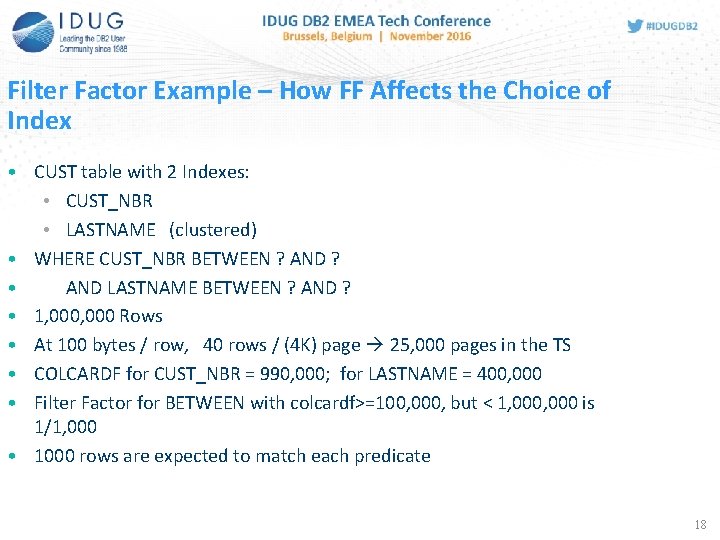
Filter Factor Example – How FF Affects the Choice of Index • CUST table with 2 Indexes: • CUST_NBR • LASTNAME (clustered) • WHERE CUST_NBR BETWEEN ? AND ? • AND LASTNAME BETWEEN ? AND ? • 1, 000 Rows • At 100 bytes / row, 40 rows / (4 K) page 25, 000 pages in the TS • COLCARDF for CUST_NBR = 990, 000; for LASTNAME = 400, 000 • Filter Factor for BETWEEN with colcardf>=100, 000, but < 1, 000 is 1/1, 000 • 1000 rows are expected to match each predicate 18

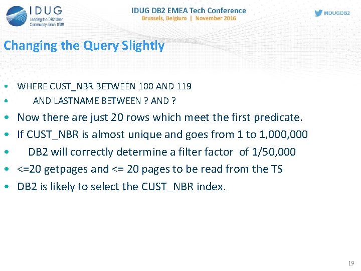
Changing the Query Slightly • WHERE CUST_NBR BETWEEN 100 AND 119 • AND LASTNAME BETWEEN ? AND ? • • • Now there are just 20 rows which meet the first predicate. If CUST_NBR is almost unique and goes from 1 to 1, 000 DB 2 will correctly determine a filter factor of 1/50, 000 <=20 getpages and <= 20 pages to be read from the TS DB 2 is likely to select the CUST_NBR index. 19

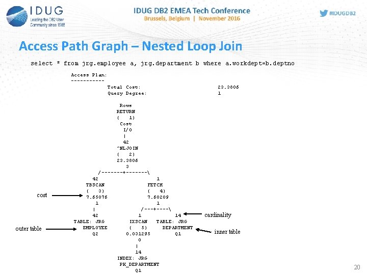
20 Access Path Graph – Nested Loop Join select * from jrg. employee a, jrg. department b where a. workdept=b. deptno Access Plan: -----Total Cost: Query Degree: 23. 3806 1 Rows RETURN ( 1) Cost I/O | 42 ^NLJOIN ( 2) 23. 3806 3 /-------+------- cost outer table 42 TBSCAN ( 3) 7. 65076 1 | 42 TABLE: JRG EMPLOYEE Q 2 1 FETCH ( 4) 7. 60209 1 /---+---- 1 14 IXSCAN TABLE: JRG ( 5) DEPARTMENT 0. 031295 Q 1 0 | 14 INDEX: JRG PK_DEPARTMENT Q 1 cardinality inner table 20

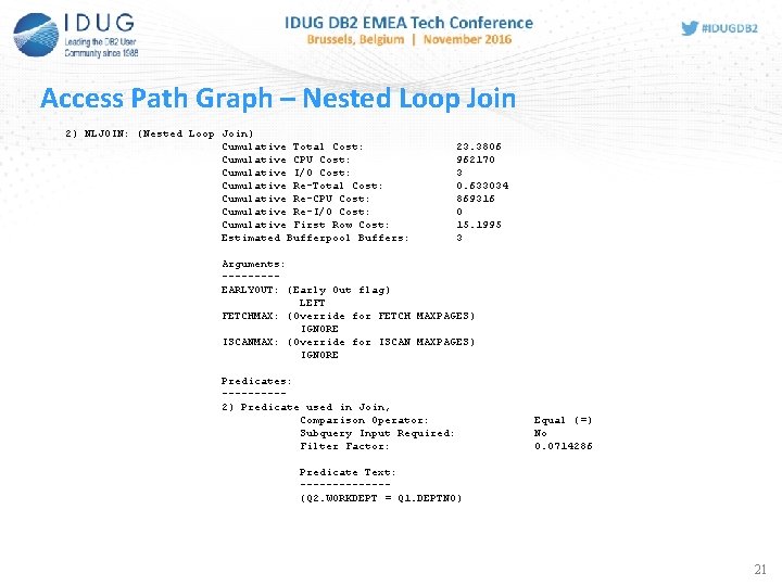
21 Access Path Graph – Nested Loop Join 2) NLJOIN: (Nested Loop Join) Cumulative Total Cost: Cumulative CPU Cost: Cumulative I/O Cost: Cumulative Re-Total Cost: Cumulative Re-CPU Cost: Cumulative Re-I/O Cost: Cumulative First Row Cost: Estimated Bufferpool Buffers: 23. 3806 962170 3 0. 633034 869316 0 15. 1995 3 Arguments: ----EARLYOUT: (Early Out flag) LEFT FETCHMAX: (Override for FETCH MAXPAGES) IGNORE ISCANMAX: (Override for ISCAN MAXPAGES) IGNORE Predicates: -----2) Predicate used in Join, Comparison Operator: Subquery Input Required: Filter Factor: Equal (=) No 0. 0714286 Predicate Text: -------(Q 2. WORKDEPT = Q 1. DEPTNO) 21

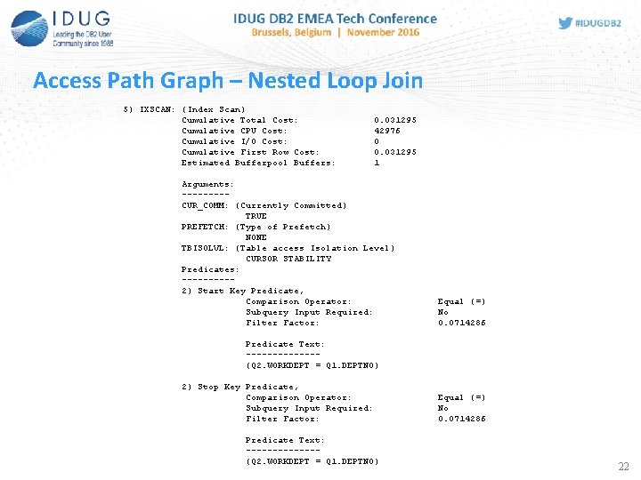
22 Access Path Graph – Nested Loop Join 5) IXSCAN: (Index Scan) Cumulative Total Cost: Cumulative CPU Cost: Cumulative I/O Cost: Cumulative First Row Cost: Estimated Bufferpool Buffers: 0. 031295 42976 0 0. 031295 1 Arguments: ----CUR_COMM: (Currently Committed) TRUE PREFETCH: (Type of Prefetch) NONE TBISOLVL: (Table access Isolation Level) CURSOR STABILITY Predicates: -----2) Start Key Predicate, Comparison Operator: Subquery Input Required: Filter Factor: Equal (=) No 0. 0714286 Predicate Text: -------(Q 2. WORKDEPT = Q 1. DEPTNO) 2) Stop Key Predicate, Comparison Operator: Subquery Input Required: Filter Factor: Predicate Text: -------(Q 2. WORKDEPT = Q 1. DEPTNO) Equal (=) No 0. 0714286 22

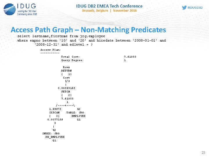
23 Access Path Graph – Non-Matching Predicates select lastname, firstnme from jrg. employee where empno between '10' and '20' and hiredate between '2008 -01 -01' and '2008 -12 -31' and edlevel = ? Access Plan: -----Total Cost: Query Degree: 7. 61055 1 Rows RETURN ( 1) Cost I/O | 0. 00595165 FETCH ( 2) 7. 61055 1 /----+---- 1. 99975 42 IXSCAN TABLE: JRG ( 3) EMPLOYEE 0. 0377159 Q 1 0 | 42 INDEX: JRG PK_EMPLOYEE Q 1 23

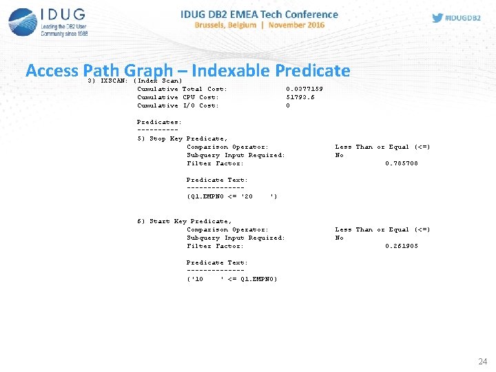
24 Access Path Graph – Indexable Predicate 3) IXSCAN: (Index Scan) Cumulative Total Cost: Cumulative CPU Cost: Cumulative I/O Cost: 0. 0377159 51793. 6 0 Predicates: -----5) Stop Key Predicate, Comparison Operator: Subquery Input Required: Filter Factor: Predicate Text: -------(Q 1. EMPNO <= '20 Less Than or Equal (<=) No 0. 785708 ') 6) Start Key Predicate, Comparison Operator: Subquery Input Required: Filter Factor: Less Than or Equal (<=) No 0. 261905 Predicate Text: -------('10 ' <= Q 1. EMPNO) 24

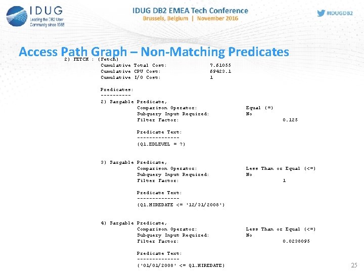
25 Access Path Graph – Non-Matching Predicates 2) FETCH : (Fetch) Cumulative Total Cost: Cumulative CPU Cost: Cumulative I/O Cost: 7. 61055 69423. 1 1 Predicates: -----2) Sargable Predicate, Comparison Operator: Subquery Input Required: Filter Factor: Equal (=) No 0. 125 Predicate Text: -------(Q 1. EDLEVEL = ? ) 3) Sargable Predicate, Comparison Operator: Subquery Input Required: Filter Factor: Less Than or Equal (<=) No 1 Predicate Text: -------(Q 1. HIREDATE <= '12/31/2008') 4) Sargable Predicate, Comparison Operator: Subquery Input Required: Filter Factor: Predicate Text: -------('01/01/2008' <= Q 1. HIREDATE) Less Than or Equal (<=) No 0. 0238095 25

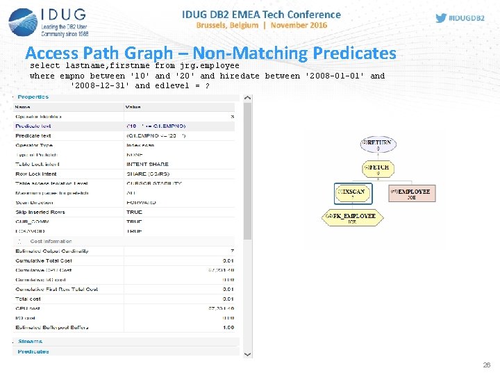
Access Path Graph – Non-Matching Predicates select lastname, firstnme from jrg. employee where empno between '10' and '20' and hiredate between '2008 -01 -01' and '2008 -12 -31' and edlevel = ? 26

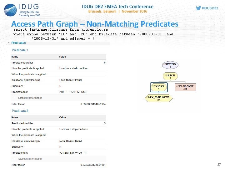
Access Path Graph – Non-Matching Predicates select lastname, firstnme from jrg. employee where empno between '10' and '20' and hiredate between '2008 -01 -01' and '2008 -12 -31' and edlevel = ? 27

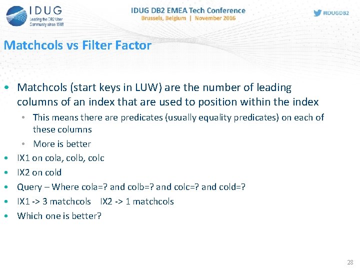
Matchcols vs Filter Factor • Matchcols (start keys in LUW) are the number of leading columns of an index that are used to position within the index • • • This means there are predicates (usually equality predicates) on each of these columns • More is better IX 1 on cola, colb, colc IX 2 on cold Query – Where cola=? and colb=? and colc=? and cold=? IX 1 -> 3 matchcols IX 2 -> 1 matchcols Which one is better? 28

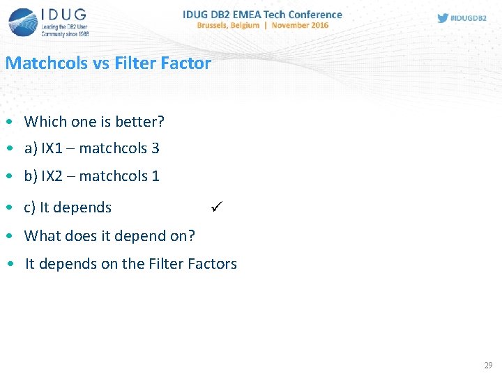
Matchcols vs Filter Factor • Which one is better? • a) IX 1 – matchcols 3 • b) IX 2 – matchcols 1 • c) It depends • What does it depend on? • It depends on the Filter Factors 29

Matchcols vs Filter Factor • The better index is the one that qualifies fewer rows • Let’s say the table was the people in the US • If IX 1 were country, state, city and the predicates were • country=‘US’ and state=‘NY’ and city=‘New York’ • 7 million rows would qualify • If IX 2 were SSN (social security number) and the predicate was • SSN = 123 -04 -0567 • 1 row would qualify. • IX 2 is much better 30

How Does the FFs affect Joins? • FFs affect joins the same way that table cardinality does • Choice of which index(es) to use • Join Method • Choice of outer / inner table • It’s better to filter more earlier 31

How Does the FFs affect Joins? • Nested Loop join is good for online transactions • Merge, Hash (LUW) joins are good for batch • OLTP – generally only a few rows are accessed • Batch – generally most of the table • Batch • Merge & Hash – 1 pass of each table. Prefetch is used • NL – if the tables are both clustered on the same key, then 1 pass with prefetch. Otherwise, random synchronous access. Each page may be read multiple times • Online • a few random I/Os are ok • HS, MS – full pass of each table 32

How Does the FFs affect Joins? • Why do we sometimes get the wrong (i. e. poorly performing) join method? • If the outer table has few selected rows, then the Optimizer may pick NL • WHERE STATUS = ? • Index on STATUS to pick up “open” orders – 100/day • But, there are only 5 STATUS values. If the table has 100 million rows, then the average is 20, 000 rows – the Optimizer picks Hash or Merge. Instead of milliseconds, the query takes 10 minutes • For a batch query, if DB 2 thinks there are only a few rows & does a NL, then instead of 10 minutes, the query may take 2 hours 33

How Do We Give DB 2 More/Better Information? • • Up to Date Statistics More Statistics Use RI (or Informational RI) Literals vs Host Variables (Parameter Markers) Reopt Statistical Views (LUW) Manually Update Statistics Selectivity Hints • LUW – Selectivity Clause • z/OS – Access Path Repository (Bind Query) 34

Literals vs Variables • Variables: • Allow one statement to be run with different values • For Dynamic SQL there is better statement reuse from the package cache / statement cache – the prepare process does not have to be repeated • Literals • Can take advantage of distribution statistics – DB 2 has more information. This can lead to a better access path, customized for the specific literal value • Range predicates also benefit from literals, even without distribution statistics • High 2 key = 100, Low 2 key = 1 WHERE COLA > 98 will have a very different FF than COLA > 2 35

Literals vs Variables • Does it Matter? Sometimes, but not always • If no column statistics at all, DB 2 uses default filter factors • If column cardinality stats, but no distribution stats, DB 2 assumes uniform distribution, so for an equals predicate the actual value doesn’t affect the access path choice. • Range predicates can use high 2 key and low 2 key for a column. • If distribution stats, then using a literal gives DB 2 even more information. A variable or parameter marker does not. 36

Literals vs Variables – Distribution Statistics • Distribution statistics are the top n most frequently occurring values for a column • • • It has the number of occurrences of that value n is configurable On LUW the default is in a db cfg parameter You can specify a different value on the runstats command If we collect the top 10 and PURCELL is not in that top 10, then DB 2 knows that it has fewer occurrences than number 10 • LUW – collecting distribution stats on all columns is common • z/OS – less common. When CPUs were slower, it was expensive so many shops did not even collect column cardinality • Who does not gather distribution stats on all columns? • Who does not gather column cardinality? 37

Literals vs Variables • But, distribution stats may not matter for all columns: • • • If the data is uniformly distributed (i. e. , not skewed) then the result is the same. Distribution stats are needed only if you have predicates on the column (i. e. you may never query by LAST_UPDATE_USERID) Column cardinality though is needed even with host variables and is strongly recommended. 5 values has a default FF=. 2 10 values has a FF=. 1 The indexes available come into play too. Example: We’ll discuss various combinations of indexes and cardinalities Select * from customer c join orders o on c. custid = o. custid where c. level = ‘GOLD’ and o. order_date = current date 38

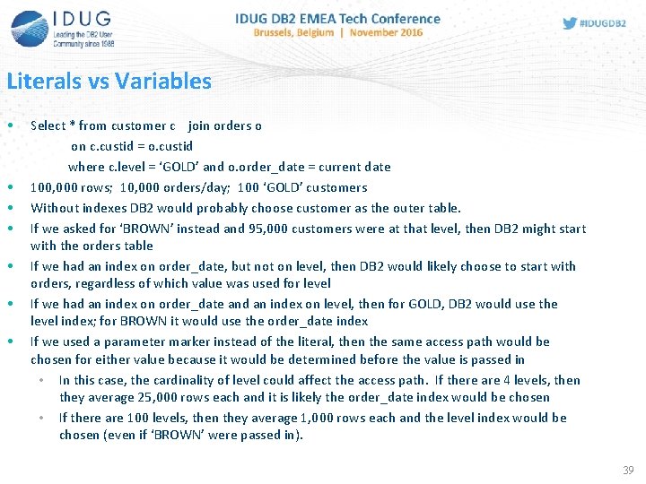
Literals vs Variables • • Select * from customer c join orders o on c. custid = o. custid where c. level = ‘GOLD’ and o. order_date = current date 100, 000 rows; 10, 000 orders/day; 100 ‘GOLD’ customers Without indexes DB 2 would probably choose customer as the outer table. If we asked for ‘BROWN’ instead and 95, 000 customers were at that level, then DB 2 might start with the orders table If we had an index on order_date, but not on level, then DB 2 would likely choose to start with orders, regardless of which value was used for level If we had an index on order_date and an index on level, then for GOLD, DB 2 would use the level index; for BROWN it would use the order_date index If we used a parameter marker instead of the literal, then the same access path would be chosen for either value because it would be determined before the value is passed in • In this case, the cardinality of level could affect the access path. If there are 4 levels, then they average 25, 000 rows each and it is likely the order_date index would be chosen • If there are 100 levels, then they average 1, 000 rows each and the level index would be chosen (even if ‘BROWN’ were passed in). 39

Literals to Parameter Markers to Literals • There are situations where we have programs that we can’t change but wish we had used parameter markers instead of literals, or vice versa • DB 2 provides optional mechanisms to do this conversion at bind or statement preparation time • Statement Concentrator / Literal Replacement • REOPT 40

Literals to Parameter Markers • Statement Cache • Allows for the reuse of dynamic SQL without DB 2 having to re-prepare the statement. This is a big performance boost for dynamic SQL. • The statements must match. Different literals will result in different statements and there will not be reuse. If there are only a few values, then each will be a different statement, but reuse should still occur • If statement is generated with literals for key fields (such as IDs), then every execution will likely be different. No reuse and the cache will be flooded – forcing out other statements that could have been reused. • Solution – Statement Concentrator 41

Literals to Parameter Markers – Statement Concentrator • Can be turned on globally with a db config parameter (LUW), or for a program via a bind parameter • You can set it as a connection property or as an Attribute on the Prepare • If the exact statement is not found in cache, DB 2 will convert literals to parameter markers and check again • Plus – statement reuse • Minus – literals not used in access path selection • Escape clause – if your statement has a mix of literals and variables, DB 2 will not convert the literals 42

Parameter Markers to Literals • Problem – program uses variables for static SQL or parameter markers for dynamic SQL because different values are passed in. But, some columns have highly skewed data • • Different values would benefit from different access paths You don’t want to convert to dynamic SQL • Solution – REOPT • REOPT is a bind option with 3 choices: • NONE – process as normal • ALWAYS – determine the access path for each execution. • ONCE – determine the access path on the first execution (the assumption here is that the first value is typical) • Is this good? Well of course that depends • PLUS – customized access paths • MINUS – execution time overhead. Access Path selection done for every execution if REOPT ALWAYS is used 43

Parameter Markers vs Literals - Recommendation • In general you should write dynamic SQL using parameter markers or host variables. • This will give you the best statement reuse and improve the performance of dynamic SQL • Use literals where it will make a difference – for low cardinality columns with a highly skewed distribution • Make sure you’ve collected distribution statistics on these columns • For software packages or where the code is already written with literals for all predicates, including ID columns, look closely at using statement concentration 44

RUNSTATS – the First Line of Defense Against Incorrect Filter Factors • Out of date stats – Runstats • Need more stats – Runstats with: • • Column cardinality FREQVAL (distribution stats) Histogram (distribution stats for ranges) COLGROUP (for columns that are correlated) • Column statistics on a subset of columns • On z/OS column stats are additive. If you ask for COL 1 and COL 2 on the first run of runstats and then ask for COL 3 on the second run, the catalog will have stats for all 3 columns • On LUW, each runstats run wipes out the column stats from prior runs. Make sure you ask for all columns and column groups you need each time you runstats 45

RUNSTATS • Why are stats often out of date? • FF stands for…… Fear Factor But a good access path today will be good tomorrow too, right? NO Things change: The number of rows Column cardinality – new values are added Column distribution Stats for related objects can become out of balance You might runstats on 1 table because of changes to the table definition, but not run it on related tables You might runstats on a new index, but not on the table Who does not run regular runstats? 46

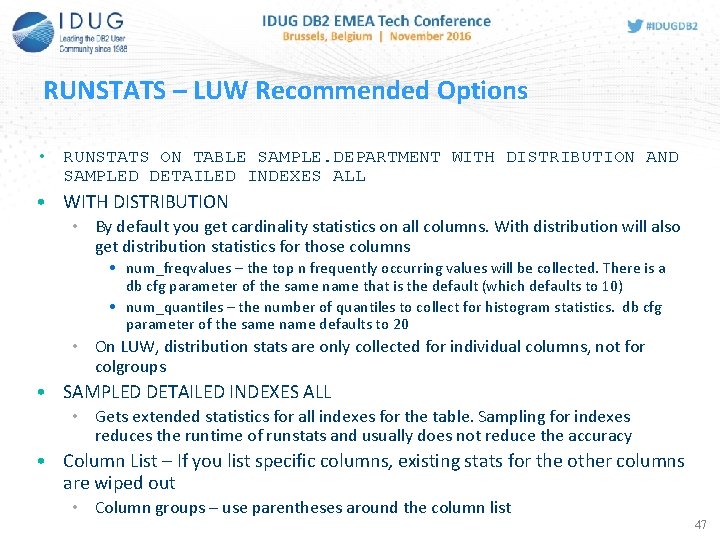
47 RUNSTATS – LUW Recommended Options • RUNSTATS ON TABLE SAMPLE. DEPARTMENT WITH DISTRIBUTION AND SAMPLED DETAILED INDEXES ALL • WITH DISTRIBUTION • By default you get cardinality statistics on all columns. With distribution will also get distribution statistics for those columns • num_freqvalues – the top n frequently occurring values will be collected. There is a db cfg parameter of the same name that is the default (which defaults to 10) • num_quantiles – the number of quantiles to collect for histogram statistics. db cfg parameter of the same name defaults to 20 • On LUW, distribution stats are only collected for individual columns, not for colgroups • SAMPLED DETAILED INDEXES ALL • Gets extended statistics for all indexes for the table. Sampling for indexes reduces the runtime of runstats and usually does not reduce the accuracy • Column List – If you list specific columns, existing stats for the other columns are wiped out • Column groups – use parentheses around the column list 47

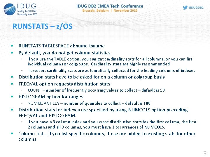
48 RUNSTATS – z/OS • RUNSTATS TABLESPACE dbname. tsname • By default, you do not get column statistics • • If you use the TABLE option, you can get cardinality stats for all columns, or you can list individual columns or colgroups. Cardinality stats are highly recommended However, cardinality stats are automatically collected for the leading columns of indexes • Distribution stats have to be asked for on a column or colgroup basis • FREQVAL option requests distribution stats • COUNT – number of frequently occurring values to collect – default is 10 • HISTOGRAM option for ranges. • NUMQUANTILES – number of quantiles to collect – default is 100 • Distribution stats for indexes are specified by using NUMCOLS option preceding FREQVAL and HISTOGRAM. • If you have a 3 column index and you want distribution stats for the first column, the first 2 columns and all 3 columns, you must have 3 occurrences of NUMCOLS. • Column List – If you list specific columns, these are added to existing stats for other columns 48

Referential Integrity • Joins are tricky. How many rows from the inner table will match each row of the outer table? • Referential Integrity helps the Optimizer. With RI, the Optimizer knows that each child row will match a single parent row if the join is on the FK columns • Unenforced RI – tells DB 2 that there is a relationship, but DB 2 doesn’t enforce that relationship. However, DB 2 can use that information to better optimize the statement. **See notes for potential issues if you have not maintained the relationship • NOT ENFORCED NOT TRUSTED – LUW 10. 5 • Prevents DB 2 from rewriting the query to eliminate one of the tables 49

Statistical Views (LUW) • A view you create and collect statistics on • It is used to capture statistics for more complex relationships – such as joins, subqueries, expressions • The statistics are used by the Optimizer when you issue a query that has a similar structure and can be matched by the Optimizer 50

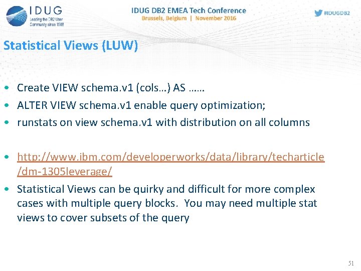
Statistical Views (LUW) • Create VIEW schema. v 1 (cols…) AS …… • ALTER VIEW schema. v 1 enable query optimization; • runstats on view schema. v 1 with distribution on all columns • http: //www. ibm. com/developerworks/data/library/techarticle /dm-1305 leverage/ • Statistical Views can be quirky and difficult for more complex cases with multiple query blocks. You may need multiple stat views to cover subsets of the query 51

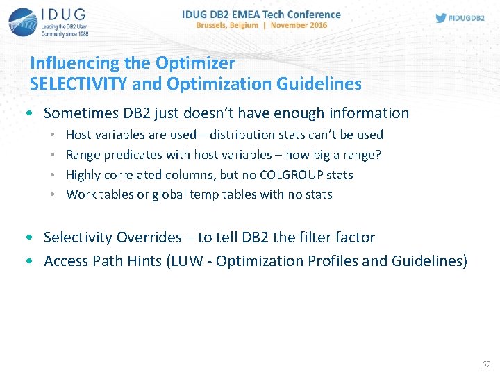
52 Influencing the Optimizer SELECTIVITY and Optimization Guidelines • Sometimes DB 2 just doesn’t have enough information • • Host variables are used – distribution stats can’t be used Range predicates with host variables – how big a range? Highly correlated columns, but no COLGROUP stats Work tables or global temp tables with no stats • Selectivity Overrides – to tell DB 2 the filter factor • Access Path Hints (LUW - Optimization Profiles and Guidelines) 52

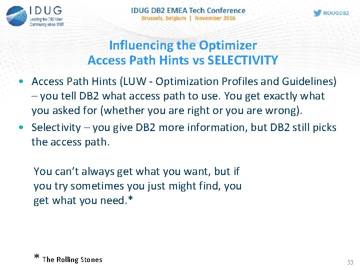
53 Influencing the Optimizer Access Path Hints vs SELECTIVITY • Access Path Hints (LUW - Optimization Profiles and Guidelines) – you tell DB 2 what access path to use. You get exactly what you asked for (whether you are right or you are wrong). • Selectivity – you give DB 2 more information, but DB 2 still picks the access path. You can’t always get what you want, but if you try sometimes you just might find, you get what you need. * * The Rolling Stones 53

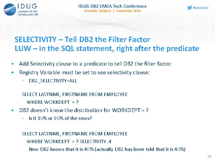
54 SELECTIVITY – Tell DB 2 the Filter Factor LUW – in the SQL statement, right after the predicate • Add Selectivity clause to a predicate to tell DB 2 the filter factor • Registry Variable must be set to use selectivity clause: • DB 2_SELECTIVITY=ALL SELECT LASTNME, FIRSTNAME FROM EMPLOYEE WHERE WORKDEPT = ? • DB 2 doesn’t know the distribution for WORKDEPT = ? • Is it 10% or 90% of the rows? SELECT LASTNME, FIRSTNAME FROM EMPLOYEE WHERE WORKDEPT = ? SELECTIVITY. 4 Now DB 2 knows that it is 40% (actually DB 2 has been told that it is 40%) 54

55 SELECTIVITY – Limitations • Not supported (yet) for all predicates. Can’t be used on BETWEEN. • Between must be split into >= and <= each with selectivity added • Selectivity can be a moving target. As the table grows and the data distribution changes, the filter factors will change too • Join predicates are a little trickier to handle • If you want to indicate that an outer row will match 1 row on average, then the selectivity will be 1/cardinality of the inner table (this assumes you know which is the inner table). The default filter factor is 1/max(colcard(t 1. joincolcard), colcard(t 2. joincolcard)) 55

SELECTIVITY z/OS – The Access Path Repository • Selectivity overrides introduced in V 11 (The APR for access path hints was introduced in V 10) • APR allows statement level hints based on matching the statement text. • Global – any statement in the system that matches • Package based – limited to a specific package • 3 types of hints • Access path hints (as was done via the plan_table) • Optimization hints (bind parameters) • Selectivity overrides 56

SELECTIVITY z/OS – The Access Path Repository • Two sets of tables are used • SYSIBM tables • SYSQUERYPREDICATE • SYSQUERYSEL • User tables to feed into the APR tables • DSN_USERQUERY_TABLE • DSN_PREDICATE_SELECTIVITY 57

SELECTIVITY z/OS – The Access Path Repository • The process: • Populate yourschema. DSN_USERQUERY_TABLE with the statement text • Do an Explain of the query. This populates the tables DSN_PREDICAT_TABLE & DSN_PREDICATE_SELECTIVITY (with the filter factor that DB 2 determined). • Update the selectivities of the predicates you want to change • The set of selectivities is a selectivity instance • You can create additional selectivity instances with different overrides for various predicates by inserting additional rows • Each instance is given a weight representing the percentage that will occur at execution time • The full set of instances is called a selectivity profile 58

SELECTIVITY z/OS – The Access Path Repository • The process: • Issue BIND QUERY • This will populate the SYSIBM tables (the APR) with the data from all queries in the DSN… tables • It is recommended to clear out these user tables of old entries before working on a new override to prevent inadvendently making an unintended change • Do an Explain of your query (or bind your package with EXPLAIN(YES) to verify the selectivity overrides were used (i. e. a match for the statement was found) and to check the access path to see if you accomplished what you intended • Execute the query and monitor the performance to see if your new access path actually is better than what you had before 59

SELECTIVITY z/OS – The Access Path Repository • The details: • http: //www 01. ibm. com/support/knowledgecenter/SSEPEK_11. 0. 0/com. ibm. db 2 z 11. doc. perf/src/tpc/db 2 z_influenceaccesspaths. dita 60

SELECTIVITY • Your query already has literals. Are selectivity overrides of any use? • Possibly. When there are literals, DB 2 can make use of distribution stats and high 2 key and low 2 key values However: • Your shop may not collect distribution stats • Your stats may be out of date – the Fear Factor strikes • Keeping stats up to date and collecting distribution stats is the preferred first step to solve filter factor problems. But, if you can’t, then overrides presents an alternative 61

SELECTIVITY Access Path Repository or Selectivity Clause Which Do You Prefer? • APR Advantages: • External to program. Can modify values without changing and redeploying the code • Can affect all occurrences of the matching statement, or just those for a particular package • Can be more detailed • Selectivity Clause Advantages: • Internal to the program. Developer is aware of its existence • Much simpler process • If the statement changes, APR must be kept in synch – redo the query in DSN_USERQUERY_TABLE and BIND QUERY (will someone notice? ) 62

Joe Geller JPMorgan Chase Joe. DB 2@aol. com Session Code: E 12 The ABCs of Filter Factors (aka Selectivity) 63