The 8 th En KF Data Assimilation Workshop

The 8 th En. KF Data Assimilation Workshop, Montreal, Canada, May 9, 2018 Localization methods for assimilating dense observations in a global LETKF Yoichiro Ota (Numerical Prediction Division/ Japan Meteorological Agency) 1

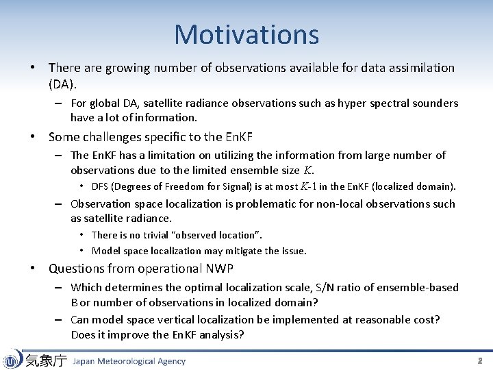
Motivations • There are growing number of observations available for data assimilation (DA). – For global DA, satellite radiance observations such as hyper spectral sounders have a lot of information. • Some challenges specific to the En. KF – The En. KF has a limitation on utilizing the information from large number of observations due to the limited ensemble size K. • DFS (Degrees of Freedom for Signal) is at most K-1 in the En. KF (localized domain). – Observation space localization is problematic for non-local observations such as satellite radiance. • There is no trivial “observed location”. • Model space localization may mitigate the issue. • Questions from operational NWP – Which determines the optimal localization scale, S/N ratio of ensemble-based B or number of observations in localized domain? – Can model space vertical localization be implemented at reasonable cost? Does it improve the En. KF analysis? 2

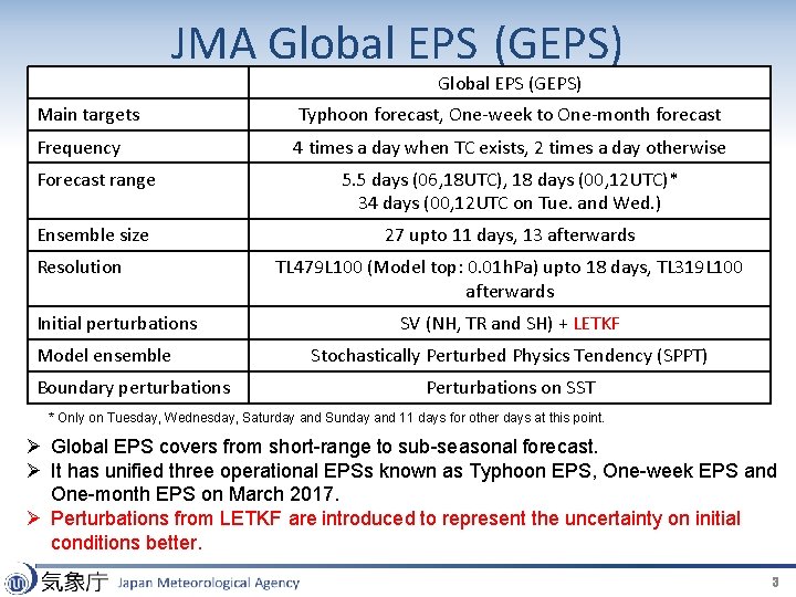
JMA Global EPS (GEPS) Main targets Typhoon forecast, One-week to One-month forecast Frequency 4 times a day when TC exists, 2 times a day otherwise Forecast range 5. 5 days (06, 18 UTC), 18 days (00, 12 UTC)* 34 days (00, 12 UTC on Tue. and Wed. ) Ensemble size 27 upto 11 days, 13 afterwards Resolution Initial perturbations Model ensemble Boundary perturbations TL 479 L 100 (Model top: 0. 01 h. Pa) upto 18 days, TL 319 L 100 afterwards SV (NH, TR and SH) + LETKF Stochastically Perturbed Physics Tendency (SPPT) Perturbations on SST * Only on Tuesday, Wednesday, Saturday and Sunday and 11 days for other days at this point. Ø Global EPS covers from short-range to sub-seasonal forecast. Ø It has unified three operational EPSs known as Typhoon EPS, One-week EPS and One-month EPS on March 2017. Ø Perturbations from LETKF are introduced to represent the uncertainty on initial conditions better. 3

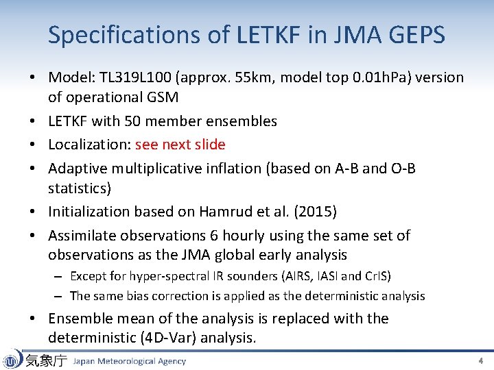
Specifications of LETKF in JMA GEPS • Model: TL 319 L 100 (approx. 55 km, model top 0. 01 h. Pa) version of operational GSM • LETKF with 50 member ensembles • Localization: see next slide • Adaptive multiplicative inflation (based on A-B and O-B statistics) • Initialization based on Hamrud et al. (2015) • Assimilate observations 6 hourly using the same set of observations as the JMA global early analysis – Except for hyper-spectral IR sounders (AIRS, IASI and Cr. IS) – The same bias correction is applied as the deterministic analysis • Ensemble mean of the analysis is replaced with the deterministic (4 D-Var) analysis. 4

Adaptive localization based on number of observations Default localization settings Ø Observation space localization based on the distance between analysis grid and observations. Ø Localization scale (1/sqrt(e)): 400 km in horizontal, 0. 4 (0. 8 for surface obs. ) scale height in vertical, 3 hours in temporal Ø For satellite radiance, maximum of normalized weighting function and gaussian function with e-holding scale of 0. 8 scale heights is used as vertical localization function*. * Normalized weighting function is used for operational LETKF Localization tested Ø Horizontal localization scale is adjusted to limit the number of observations pl in local analysis for each observation type • Shorter localization scale is applied to the dense observations. • pl is tuned so that sum of the localization function in local analysis becomes approximately half of the default setting (that is equivalent to set the horizontal localization scale to 300 km uniformly). • Vertical and temporal localization functions are the same as the default settings. 5

Experimental settings • Model: TL 319 L 100 (approx. 55 km, model top 0. 01 h. Pa) version of operational GSM • LETKF with 50 member ensembles • Adaptive multiplicative inflation (based on A-B and O-B statistics) • Initialization based on Hamrud et al. (2015) • Assimilate observations 6 hourly using the same set of observations as the JMA global cycle analysis (without hyper spectral sounders) • Experiments – CNTL: default localization settings – ADAP: adaptive localization scale – H 300: horizontal localization scale is set to 300 km • Period: From July 10, 2016 to September 11, 2016 (Forecasts are verified for August 2016) • Bias correction coefficients of 4 DVar (Var. BC) are used, but the analysis ensemble mean is not replaced with the 4 DVar analysis. 6

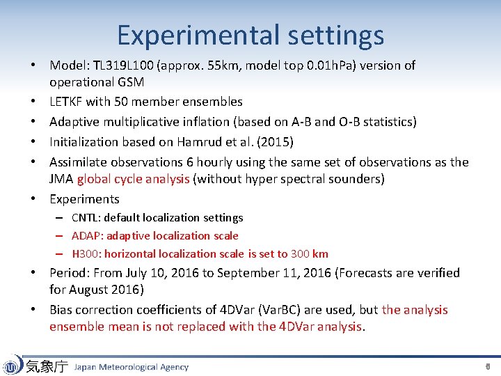
DFS (Degrees of Freedom for Signal) CNTL H 300 ADAP Period August 2016 Ensemble-based DFS by Liu et al. (2009) DFS by Lupu et al. (2011) Ø DFS statistics by two different methods are mostly consistent. Ø DFS values of both ADAP and H 300 are larger than that of CNTL. More information is extracted from the observations 7

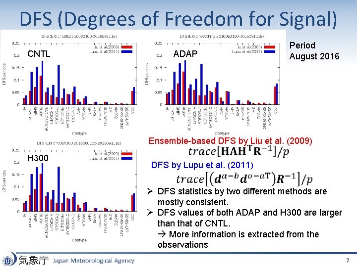
O-B statistics AMSU-A MHS Relative changes [%] in standard deviation of O-B for AMSU-A and MHS. 0 ADAP-CNTL 12% 0 6% H 300 -CNTL Ø O-B of H 300 is smaller than that of ADAP. • Localization scale adjustment based on observation numbers is not better than simple uniform localization scale change. Ø O-B of H 300 and ADAP for AMSU-A are larger than that of CNTL. On the other hand, O-B of H 300 for MHS is smaller than that of CNTL. • Suggesting optimal localization scale for MHS (humidity sensitive ch) is shorter than that for AMSU-A (temperature sensitive ch). Ø For AMSU-A, O-B of H 300 and ADAP are degraded especially on stratosphere which suggests wider horizontal localization is preferable in the stratosphere. 8

O-B statistics (cont. ) AMSU-A MHS Relative changes [%] in standard deviation of O-B for AMSU-A and MHS. * Humidity sensitive observations: MHS, ATMS (ch 18 -22), SSMIS (ch 9 -11), GMI, AMSR 2, SAPHIR, CSR, RH (radiosonde) Q 300 -CNTL Ø When horizontal localization scale of humidity sensitive observations* is set to 300 km (Q 300), O-B of both AMSU-A and MHS are decreased. • One possibility is that the ensemble-based B of humidity is noisier than those of other variables. Thus, shorter horizontal localization scale is preferable. Optimal localization scale is likely determined by the S/N ratio of ensemblebased background error covariance, not by the observation density (at least with current observation coverage). 9

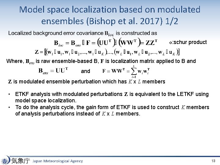
Model space localization based on modulated ensembles (Bishop et al. 2017) 1/2 o: schur product Where, Bens is raw ensemble-based B, F is localization matrix applied to B and Z is modulated ensemble perturbation which has K x L members • ETKF analysis with modulated perturbations Z is equivalent to the LETKF using model space localization. • To do the analysis cycle, the gain form of ETKF is used to construct K members of analysis perturbations instead of K x L members. 13

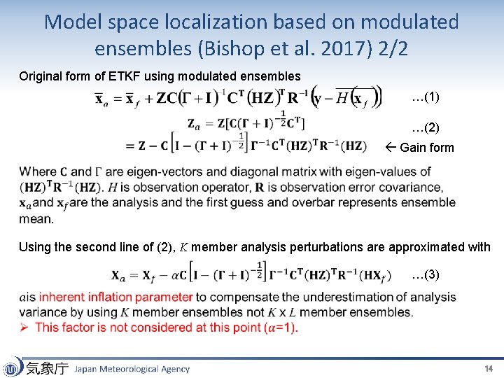
Model space localization based on modulated ensembles (Bishop et al. 2017) 2/2 Original form of ETKF using modulated ensembles …(1) …(2) Gain form Using the second line of (2), K member analysis perturbations are approximated with …(3) 14

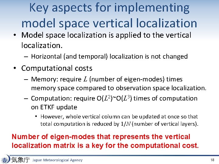
Key aspects for implementing model space vertical localization • Model space localization is applied to the vertical localization. – Horizontal (and temporal) localization is not changed • Computational costs – Memory: require L (number of eigen-modes) times memory space compared to observation space localization. – Computation: require O(L 2)~O(L 3) times of computation on ETKF update • However, whole vertical column can be updated at once so that total computation is reduced by 1/N (number of vertical layers). Number of eigen-modes that represents the vertical localization matrix is a key for the computational cost. 15

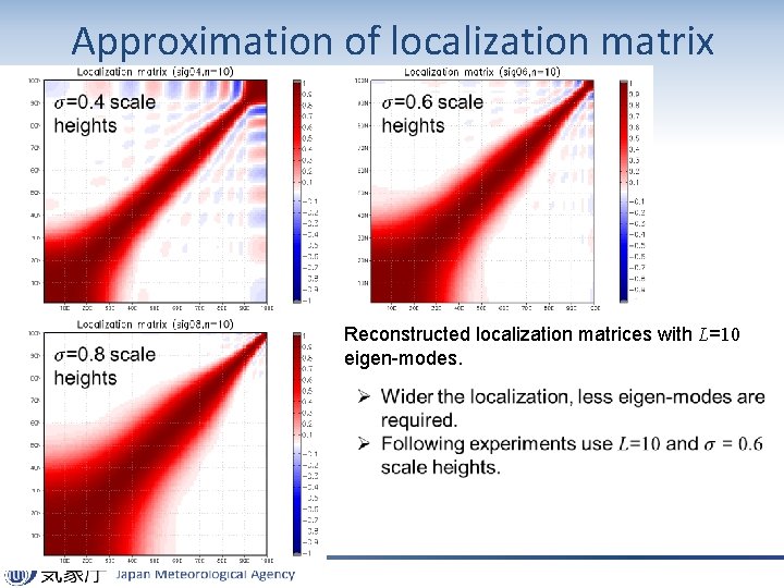
Approximation of localization matrix Reconstructed localization matrices with L=10 eigen-modes.

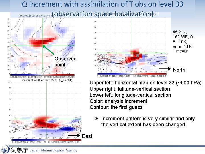
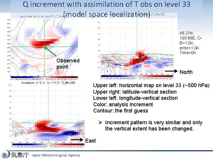
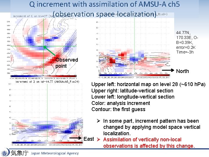
Q increment with assimilation of T obs on level 33 (observation space localization) 45. 21 N, 169. 88 E, OB=1. 0 K, error=1. 0 K Time=0 h Observed point North Upper left: horizontal map on level 33 (~500 h. Pa) Upper right: latitude-vertical section Lower left: longitude-vertical section Color: analysis increment Contour: the first guess Ø Increment pattern is very similar and only the vertical extent has been changed. East

Q increment with assimilation of T obs on level 33 (model space localization) 45. 21 N, 169. 88 E, OB=1. 0 K, error=1. 0 K Time=0 h Observed point North Upper left: horizontal map on level 33 (~500 h. Pa) Upper right: latitude-vertical section Lower left: longitude-vertical section Color: analysis increment Contour: the first guess Ø Increment pattern is very similar and only the vertical extent has been changed. East

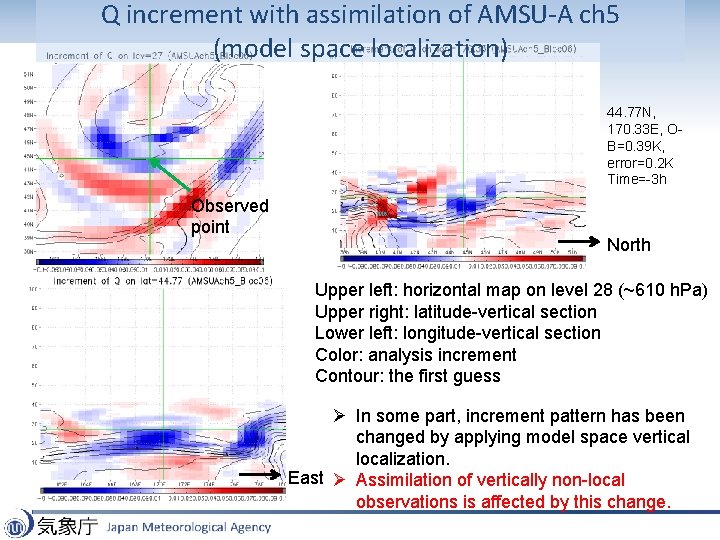
Q increment with assimilation of AMSU-A ch 5 (observation space localization) 44. 77 N, 170. 33 E, OB=0. 39 K, error=0. 2 K Time=-3 h Observed point North Upper left: horizontal map on level 28 (~610 h. Pa) Upper right: latitude-vertical section Lower left: longitude-vertical section Color: analysis increment Contour: the first guess Ø In some part, increment pattern has been changed by applying model space vertical localization. East Ø Assimilation of vertically non-local observations is affected by this change.

Q increment with assimilation of AMSU-A ch 5 (model space localization) 44. 77 N, 170. 33 E, OB=0. 39 K, error=0. 2 K Time=-3 h Observed point North Upper left: horizontal map on level 28 (~610 h. Pa) Upper right: latitude-vertical section Lower left: longitude-vertical section Color: analysis increment Contour: the first guess Ø In some part, increment pattern has been changed by applying model space vertical localization. East Ø Assimilation of vertically non-local observations is affected by this change.

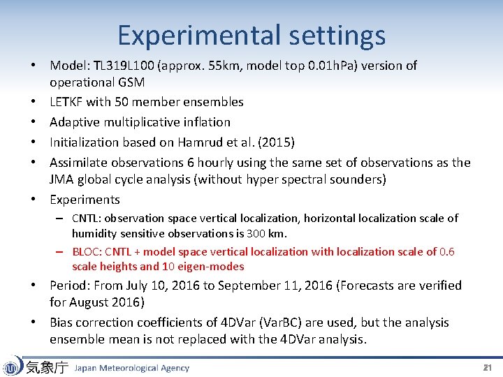
Experimental settings • Model: TL 319 L 100 (approx. 55 km, model top 0. 01 h. Pa) version of operational GSM • LETKF with 50 member ensembles • Adaptive multiplicative inflation • Initialization based on Hamrud et al. (2015) • Assimilate observations 6 hourly using the same set of observations as the JMA global cycle analysis (without hyper spectral sounders) • Experiments – CNTL: observation space vertical localization, horizontal localization scale of humidity sensitive observations is 300 km. – BLOC: CNTL + model space vertical localization with localization scale of 0. 6 scale heights and 10 eigen-modes • Period: From July 10, 2016 to September 11, 2016 (Forecasts are verified for August 2016) • Bias correction coefficients of 4 DVar (Var. BC) are used, but the analysis ensemble mean is not replaced with the 4 DVar analysis. 21

-20% +20% Relative changes [%] in number of used observations for AMSU-A and MHS. Ø The first guess spread has been decreased by 10 -20% in most layers. Ø O-B of observations on stratosphere has been decreased and more observations are assimilated. Ø Reduction of the first guess spread seems too large compared to the reduction of O-B. AMSU-A -5% 0 MHS Relative changes [%] in standard deviation of O-B for AMSU-A and MHS. AMSU-A Relative change [%] of the first guess spread of U on 250 h. Pa (BLOC compared to CNTL) MHS Analysis changes 0 +2. 8% The first guess on stratosphere seems to be improved by model space vertical localization. O-A is mostly increased (not shown) suggesting the reduction of B is too large. 22

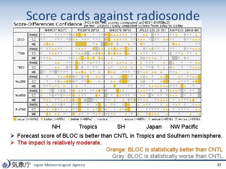
Score cards against radiosonde NH Tropics SH Japan NW Pacific Ø Forecast score of BLOC is better than CNTL in Tropics and Southern hemisphere. Ø The impact is relatively moderate. Orange: BLOC is statistically better than CNTL Gray: BLOC is statistically worse than CNTL 23

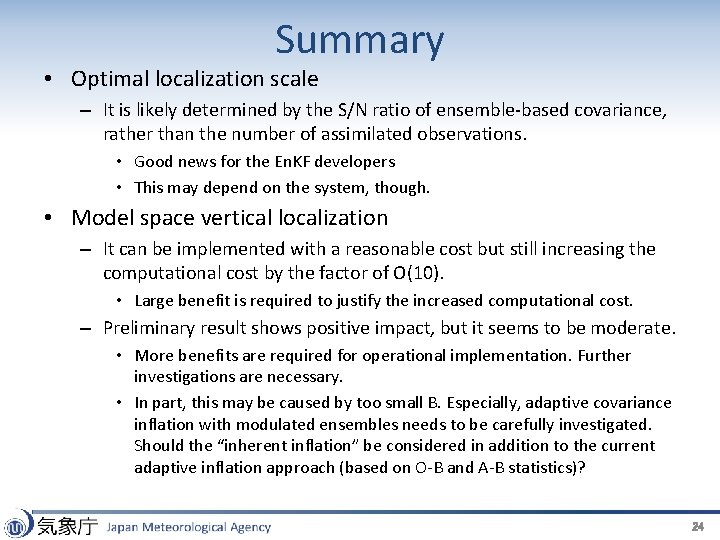
Summary • Optimal localization scale – It is likely determined by the S/N ratio of ensemble-based covariance, rather than the number of assimilated observations. • Good news for the En. KF developers • This may depend on the system, though. • Model space vertical localization – It can be implemented with a reasonable cost but still increasing the computational cost by the factor of O(10). • Large benefit is required to justify the increased computational cost. – Preliminary result shows positive impact, but it seems to be moderate. • More benefits are required for operational implementation. Further investigations are necessary. • In part, this may be caused by too small B. Especially, adaptive covariance inflation with modulated ensembles needs to be carefully investigated. Should the “inherent inflation” be considered in addition to the current adaptive inflation approach (based on O-B and A-B statistics)? 24

References • Bishop, C. H. , J. S. Whitaker and L. Lei, 2017: Gain form of the Ensemble Transform Kalman Filter and its relevance to satellite data assimilation with model space ensemble covariance localization. Mon. Wea. Rev. , 145, 4575 -4592. • Hamrud, M. Monavita and L. Isaksen, 2015: En. KF and hybrid gain ensemble data assimilation. Part I: En. KF implementation. Mon. Wea. Rev. , 143, 4847 -4864. • Liu, J. , E. Kalnay, T. Miyoshi and C. Cardinali, 2009: Analysis sensitivity calculation in an ensemble Kalman filter. Q. J. R. Meteorol. Soc. , 135, 1842 -1851. • Lupu, C. , P. Gauthier and S. Laroche, 2011: Evaluation of the Impact of Observations on Analyses in 3 D- and 4 D-Var Based on Information Content. Mon. Wea. Rev. , 139, 726 -737. 25

Backups 26

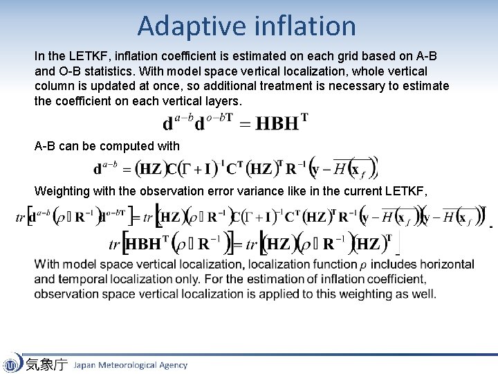
Adaptive inflation In the LETKF, inflation coefficient is estimated on each grid based on A-B and O-B statistics. With model space vertical localization, whole vertical column is updated at once, so additional treatment is necessary to estimate the coefficient on each vertical layers. A-B can be computed with Weighting with the observation error variance like in the current LETKF,