The 2 k Factorial Design Introduction The special

The 2 k Factorial Design

Introduction • The special cases of the general factorial design • k factors and each factor has only two levels • Levels: – quantitative (temperature, pressure, …), or qualitative (machine, operator, …) – High and Low – A complete replicate of this design requires 2 2 = 2 k observations

• Assumptions: (1) The factor is fixed. (2) The design is completely randomized. (3) The usual normality assumptions are satisfied. • Additional assumption: The response is approximately linear over the range of the factor levels chosen. • Useful in the early stages of experimental work when there are many factors to be investigated. • Wildly used in factor screening experiments

The 22 Factorial Design • Two factors, A and B, and each factor has two levels, low and high. • Example: the concentration of reactant (15% and 25%) v. s. the amount of the catalyst (one bag and two bags)

• “-” And “+” denote the low and high levels of a factor, respectively. • Geometrically, the four treatment combinations form the corners of a square and are represented by lowercase letters. • The high level of any factor in the treatment combination is denoted by the corresponding lowercase letter and the low level of a factor in the treatment combination is denoted by the absence of the corresponding letter.

• (1), a, b and ab present the total of all n replicates taken at the treatment combination. • (1) is used to denote both factors at the low level. • a represents the treatment combination of A at the high level and B at the low level. • b represents the treatment combination of A at low level and B at the high level. • ab represents the treatment combination of A at high level and B at the high level. • Average effect of a factor can be defined as : “The change in response produced by a change in the level of that factor averaged over the levels of the other factors. ”

• The main effects:

• The interaction effect AB is defined as the average difference between the effect of A at the high level of B and the effect of A at the low level of B. • The interaction effect:

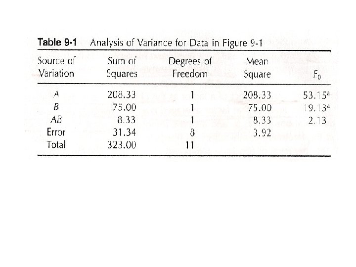
• From the example, the average effects can be estimated as follows. A = 8. 33, B = -5. 00 and AB = 1. 67 • The magnitude and direction of the factor effects are examined to determine which variables are likely to be important. • The analysis of variance can be used to confirm the interpretation. • The total effects:

• Sum of squares:

Response: Conversion ANOVA for Selected Factorial Model Analysis of variance table [Partial sum of squares] Sum of Source Squares Model 291. 67 A 208. 33 B 75. 00 AB 8. 33 Pure Error 31. 33 Cor Total 323. 00 DF 3 1 1 1 8 11 Mean Square 97. 22 208. 33 75. 00 8. 33 3. 92 F Value 24. 82 53. 19 19. 15 2. 13 Prob > F 0. 0002 < 0. 0001 0. 0024 0. 1828 Std. Dev. Mean C. V. 1. 98 27. 50 7. 20 R-Squared Adj R-Squared Pred R-Squared 0. 9030 0. 8666 0. 7817 PRESS 70. 50 Adeq Precision 11. 669 The F-test for the “model” source is testing the significance of the overall model; that is, is either A, B, or AB or some combination of these effects important?

• The contrast coefficients for estimating the interaction effect are just the product of the corresponding coefficients for the two main effects. • I represents the total or average of the entire experiment.

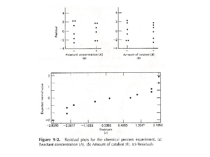
Residual Analysis • Compute the residuals via a regression model which is and = coded variables = +1 or -1 = regression coefficients = the residual From the example,

At the high level of the concentration, = +1 At the low level of the concentration, = -1 At the high level of the catalyst, = +1 At the low level of the catalyst, = -1 • The fitted regression model is • The interception is the grand average of all observations and the regression coefficients are one-half the corresponding factor effect estimates. • The residual can be computed from.

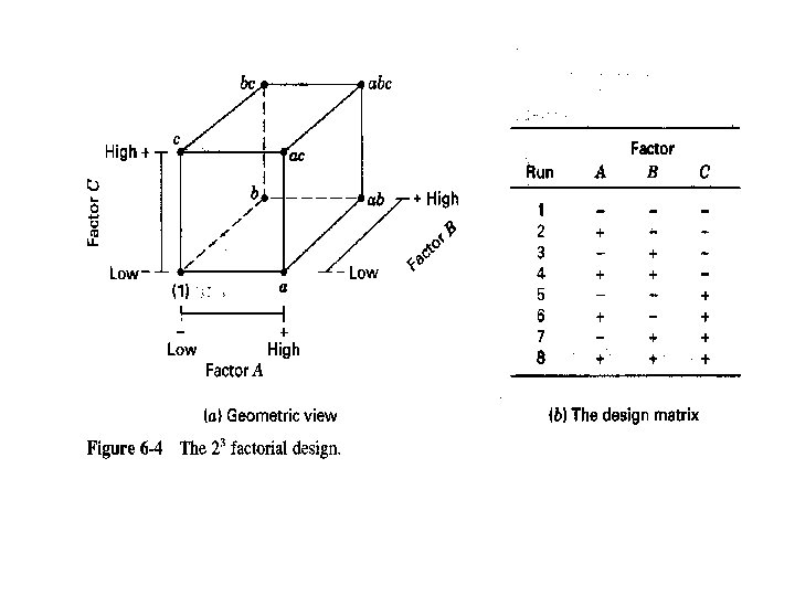
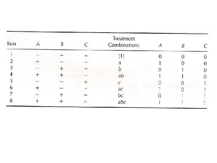
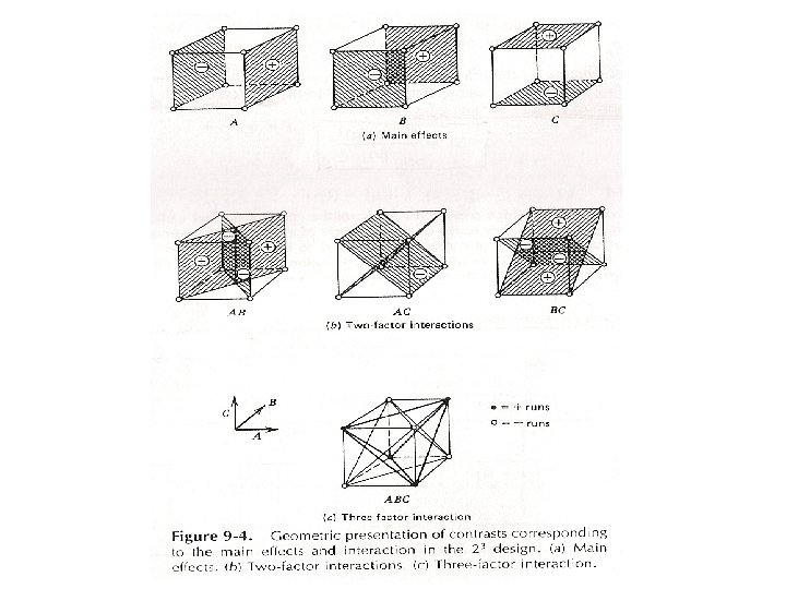
The 23 Design • Three factors, A, B and C, and each factor has two levels. • 23 factorial design • Eight treatment combinations: (1), a, b, ab, c, ac, bc, abc • There are n observations taken at each treatment combination.

• Estimate main effects:

• Estimate two-factor interaction effects: the difference between the average A effects at the two levels of B

• Three-factor interaction effect: • In all above equations, the quantities in brackets are contrasts in the treatment combinations. • Signs for the main effects are determined by associating a plus (+) with the high level and a minus (-) with the low level.

• Once the signs for the main effects have been established, the signs for the interaction effects (columns) can be obtained by multiplying the appropriate preceding columns, row by row.

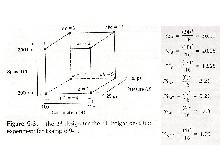
• Contrast: – Every column has an equal number of plus and minus signs. – The sum of the products of the signs in any two columns = 0. – I is an identity element. – The product of any two columns yields another column. • Sum of squares for any effects can be computed from

Example: A = carbonation, B = pressure, C = speed, y = fill deviation

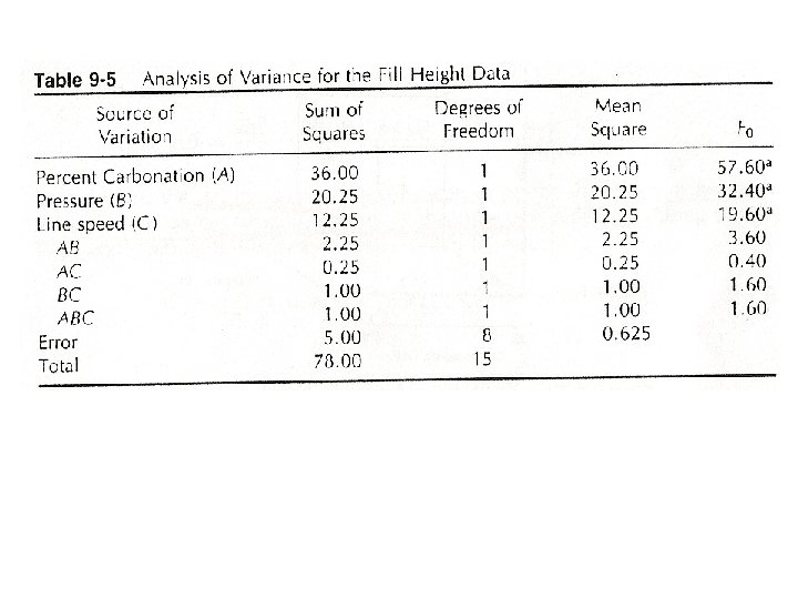
• ANOVA Summary – Full Model Response: Fill-deviation ANOVA for Selected Factorial Model Analysis of variance table [Partial sum of squares] Sum of Source Squares Model 73. 00 A 36. 00 B 20. 25 C 12. 25 AB 2. 25 AC 0. 25 BC 1. 00 ABC 1. 00 Pure Error 5. 00 Cor Total 78. 00 DF 7 1 1 1 1 8 15 Mean Square 10. 43 36. 00 20. 25 12. 25 0. 25 1. 00 0. 63 F Value 16. 69 57. 60 32. 40 19. 60 3. 60 0. 40 1. 60 Prob > F 0. 0003 < 0. 0001 0. 0005 0. 0022 0. 0943 0. 5447 0. 2415 Std. Dev. Mean C. V. 0. 79 1. 00 79. 06 R-Squared 0. 9359 Adj R-Squared Pred R-Squared 0. 8798 0. 7436 PRESS 20. 00 Adeq Precision 13. 416

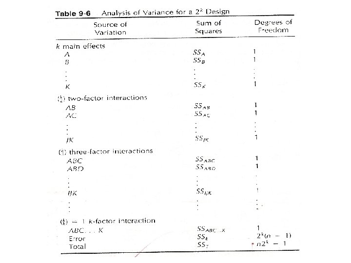
The General 2 k Design • k factors and each factor has two levels. • There are n observations taken at each treatment combination. • The complete model contains 2 k -1 effects. k main effects

• The treatment combinations may be written in standard order by introducing the factors one at a time, with each new factor being successively combined with those that precede it. • The standard order for a 24 design: (1), a, b, ab, c, ac, bc, abc, d, ad, bd, abd, cd, acd, bcd, abcd • To estimate an effect or to compute the sum of squares for an effect, the contrast associated with that effect must be determined first. • The contrast for effect AB…K can be determined from

• The sign in each set of parentheses is negative (-) if the factor is included in the effect and positive (+) if the factor is not included. • The term “ 1” is replaced by (1). For example, the contrast of A effect for 22 design can be found as follows: • Once the contrasts for the effects have been computed, the effects and the sum of squares can be determined from