The 2 D Projective Plane Points and Lines

The 2 D Projective Plane Points and Lines

The 2 D projective plane A point in a plane is represented by (x, y) in R 2 (x, y) is also a vector Homogeneous representation point ( x 1, x 2 , x 3 ) x= x 1/ x 3 y = x 2/ x 3 One representation of a point is ( x, y, 1 )

Lines and points Line ax + by +c = 1 • ( x, y, 1) ( a, b, c)T =0 • x. Tl = 0 • l = (a, b, c)T l’ = (a’, b’, c’)T Define the vector x = l x l’ Intersection of 2 lines Where x is a cross product

Cross products • From the identity l. (l x l’) = l’. (l x l’) = 0 l. Tx = l’Tx = 0 • Thus x is a point lying in both l and l’ which is the intersection of two lines • Line joining 2 points l = x x x’

Ideal points and line at infinity 1 • Intersection of parallel lines l = (a, b, c) and l’ = (a, b, c’) are parallel l x l’ = (c’ – c)( b, -a, 0)T • Ignoring scale, it is a point ( b, -a, 0)T with inhomogeneous coordinates (b/0, -a/0)T It is a point at infinity where the lines meet. It is not a finite point in R 2

Ideal points and line at infinity 2 • The points with last coordinate x 3 = 0 are known as ideal points, or points at infinity. Note that this set lies on a single line , the line at infinity linf = ( 0, 0, 1)T as ( 0, 0, 1) (x 1 , x 2 , 0) = 0 A line l =( a, b, c)T intersect the line at infinity in the ideal point ( b, -a, 0)T (b, -a) T represent the line’s direction

Ideal points and line at infinity 3 • The line at infinity can be thought of as the set of directions of all lines in the plane. • One may argument R 2 by adding points with the last coordinate x 3 = 0, • The resulting space is p 2 is named the projective space • The geometry of p 2 is known as projective geometry

A model of projective plane • A fruitful way of thinking : p 2 is a set of rays in R 3. Each vector k( x 1, x 2, x 3)T as k varies forms a ray pass through the origin. A ray can be thought of a point in p 2 In this model , the lines in p 2 are planes passing through the origin

Points and lines of p 2 are represented as rays and planes through the origin

A model of the projective plane • Points and lines of p 2 are represented by rays and planes respectively, through the origin in R 3. • x 1 x 2 - plane represents the line at infinity linf Lines in x 1 x 2 plane represent ideal points

Projective plane model 2 • Two non-identical rays lie on exactly one plane, and any two planes intersect at one ray. • This is analogue of two distinct points define a line and two lines meet always intersect at a point. • Points and lines may be obtained by intersecting rays and planes by the plane x 3 = 1 • The rays representing ideal points and the plane representing linfinity are parallel to the plane x 3 =1

Duality Principle • To any theorem of 2 –dimensional projective geometry, there corresponds a dual theorem, which may be derived by interchanging the roles of points and lines in the original theorem

Conics and Dual conics • A conic is a curve described by a seconddegree equation in the plane. • In Euclidean geometry, conics are of 3 main types: hyperbola, ellipse and parabola • In 2 D projective geometry all nondegenerate conics are equivalent under projective transformations

Equation of conics • In inhomogeneous coordinates, a conic is given by • ax 2 + bxy + cy 2 + dx + ey + f = 0 • Let x = x 1/x 3 , y = x 1/x 3 , Then • ax 12 + bx 1 x 2 + cx 12 + dx 1 x 3 +ex 2 x 3 +fx 32 =0

Conics • In matrix form • x. T C x = 0 • C= where

Five point define a conic • C is symmetric and only the ratios of the matrix elements are important. C has 5 degrees of freedom Put x 3 =1. If C passes through xi, yi, , then ( xi 2 xi yi yi 2 xi yi 1) c =0 where c = ( a, b, c, d, e, f)T is the conic represented as a 6 -vector

Constraints from 5 points c = 0

Tangent lines to conics • The line l tangent to a conic C at a point x on C is given by l = Cx

Dual Conics • There exist a dual conic C* which defines an equation on lines. • A line l tangent to the conic C satisfies • l. T C* l = 0 • C* is the adjoint matrix of C • For a non-singular symmetric matrix C* = C-1

Degenerated conics • If C is not of full rank, then the conic is termed degnerate. Degenerate point conics include 2 lines ( rank 2) and a repeated line (rank 1) • C = l m. T + m l T • Is composed of two lines l and m

Projective transformations • A projectivity is an invertible mapping h from p 2 to itself such that three points x 1, x 2 and x 3 lie on the same line if and only if h (x 1), h(x 2) and h( x 3) do. Projectivities form a group. Projectivity is also called A projective transformation or a homography

Projective transformations 2 • A mapping h : p 2 is a projectivity if and only if there exists a non-singular 3 x 3 matrix H such that for any point in p 2 represented by a vector x is true that h(x) = H x. Any point in p 2 is represented as a homogenous 3 vector x, and Hx is a linear mapping of the homogeneous coordinates

Central projection maps points to points and lines to lines

Definition • A planar projective transform is represented by a non-singular 3 x 3 matrix H • where x’ = H x

Removing the projective distortion from the perspective image of a plane • Compute projective transform from point correspondence: x’=Hx

Four point correspondences lead to 8 such linear equations on H • Four points gives 8 constraints are used to computing H. • The points must be in general position: no 3 points are collinear. • x= H-1 x’ Remove projective distortion

Three remarks on computing H • Knowledge of camera parameters or the pose of plane are not required • 4 points are not always necessary. Alternative approach requires less information. • Superior methods of computing projective transform are described later

Removing the projective distortion from a perspective image of a plane • H between image and plane can be computed without knowing the camera parameters

The projective transformation between two images induced by a world plane

The projective transformation between two images with the same camera centre

The projective transformation the image of a plane and the image of its shadow onto another plane

Transformation of lines • Under a point transformation x’ = H x, • Given xi lies on l , x’ will lie on a transformed line l’ =H-T l • In this way, l’T xi’ = l. T H-1 Hxi =0 •

Transformation of conics x = H-1 x’ x. T =x’T H-T x. T Cx = x’T H-TC H-1 x’ = x’T C’ x’ A conic C transform to C’ = H-T C H-1 A dual conic transform to C*’ = HC*HT

Distortion arising under central projection Images of a tiled floor: Similarity, Affine, Projective

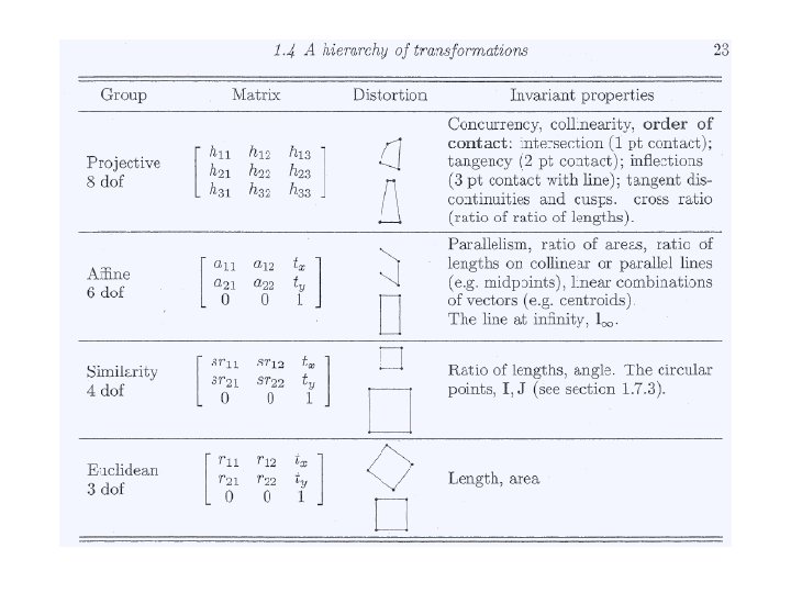
A hierarchy of transformations • Class 1: Isometries • An isometry is represented as where e = 1 or -1

Euclidean transformation • If e = 1, the isometry is orientation- preserving and is an Euclidean transformation If e = -1, the isometry reverse orientation HE is a planar Euclidean transformation with R a 2 x 2 rotation matrix

Groups and orientation • An isometry is orientation-preserving if R has determinant 1. The isometries form a group. • This also applies to the cases of • Similarity and affine transformation

Class ll: Similarity transformations

Class lll: Affine transformation

Decomposing an affine matrix A • A = R (q) R(-f) D R(f) • Where R (q) and R(f) are rotation by q and f respectively. D is a diagonal matrix. • This follows from the SVD where U and V are orthogonal matrices • A = (UVT)(VDVT)= R (q) (R(-f) D R(f))

Invariants • (i) parallel lines • (ii) Ratio of lengths of parallel line segments • (iii) Ratio of areas

Distortion arising from a planar affine transformation

Class l. V: Projective transformation • Vector v is a 2 -vector and v is a scaler. The matrix has 9 elements with only their ratio significant.

Comparing affine and projective transformations Ideal points are mapped to finite points in projective transformations

Decomposition of a projective transformation H • A is a non-singular matrix given by A=s. RK+tv. T • And K is an upper triangular matrix normalized as • Det K =1

An example

The projective Geometry of 1 D

A few comments on the cross ratio

Cross ratio: alternative definition • Cross ratio expressed as ratio of ratios of lengths: • Let A, B, C, and D be 4 collinear points. The basic invariant of any homology is the cross ratio • (A, B, C, D) = • The points at infinity

Concurrent lines • A configuration of concurrent lines is dual to collinear points on a line. • This means the concurrent lines on a plane also have the geometry p 1. • In particulars, 4 concurrent lines have across ratio as shown in the following slide

Projective transformation between lines There are 4 sets of four collinear points. The cross ratio is an invariant under projectivity

Concurrent lines; dual to collinear points on a line

Recovery of affine and metric properties from images • It is noted that the projective distortion in the perspective image of a plane is removed by specifying 4 points. ( 8 dof) • However, only 4 dof is required to specified in order to determine metric properties. • These 4 dof are given physical substance by associating them with geometric objects: • The line at infinity linf( 2 dof) and the circular points (2 dof)

The line at infinity linf is a fixed line under the projective transformation H if and only if H is an affinity. • Once the line at infinity linf is specified, the projective distortion is removed to give affine image. • The affine distortion is removed once the image of the circular points are specified.

Recovery of affine properties from images • A transform H can be computed which transforms the identified linf to its canonical position linf = ( 0, 0, 1)T. Then H may be applied to every point to rectify the image. The H is given by ( HA is any affine matrix)

Affine rectification

Affine rectification via the vanishing line

Equal distance ratios on a line to determine the point at infinity 1 inf

Equal distance ratios on a line to determine the point at infinity 2

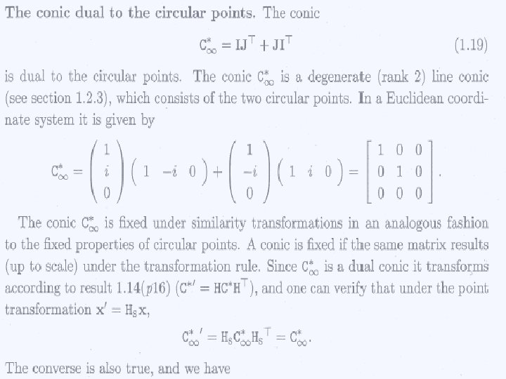
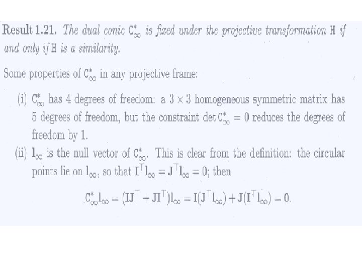
Circular points and their dual

Notes on circular points

Notes on circular points Algebraically, the circular points are the orthogonal directions of Euclidean geometry, (1, 0, 0)T and (0, 1, 0)T packaged into a single complex conjugate entity l = (1, 0, 0)T + i (0, 1, 0)T

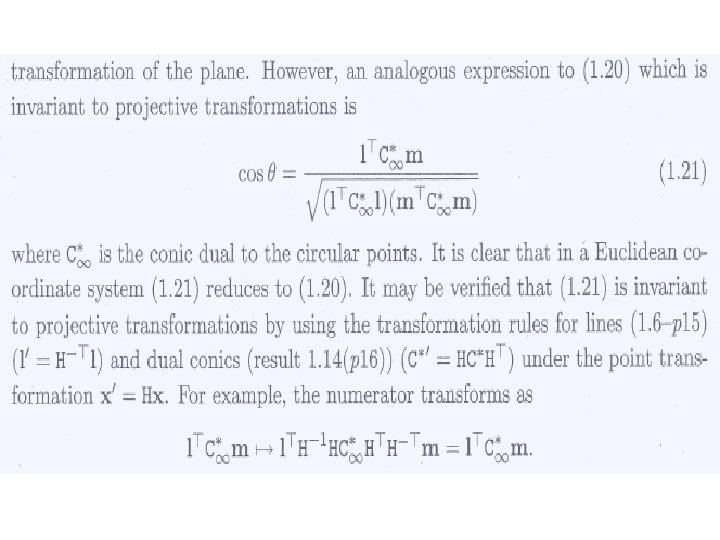
Angles on the projective plane

Some results • 1. 22 once the conic C*inf is identified on the projective plane, then Euclidean angle can be measured • As a corollary • 1. 23 Lines l and m are orthogonal if

Length ratios

Recovery of metric properties from images • Same as recovering affine properties by specifying linf , metric properties can be recovered from an image of a plane by transforming the circular points to their canonical position. • A projective transform H that maps the images of the circular points to their canonical positions at

Length ratios

Metric rectification using Using

Results

Metric rectification via orthogonal lines l

Example 1. 25 Metric rectification 1 • Suppose the line l’ and m’ in the affinely rectified image corresponding to an orthogonal pair l and m on the world plane. Using v=0, and the result:

Metric rectification 1 (cond) • It is a linear constraint on the matrix S = KKT • S is symmetric and with 3 parameters with • 2 dof ( no overall scaling). Thus • where s = (s 11 , s 12 , s 22 )

Metric rectification via orthogonal lines ll

Example 1. 26 Metric rectification ll using 5 line pairs • We start from the original perspective image and l and m are images of orthogonal lines in a world plane. Then from the result • This provides a linear constraint on the conic

The pole-polar relationship

More properties of conics • A point x and conic C define a line l = Cx. The line is called the polar of x with respective to C, and point x is the pole of l with respect to C. The polar line l = Cx of the point x with respect to C intersects the conic in two points. The two lines tangent to C at these points intersect at x

Conjugate points • If the point y is on the line l = C x , then, y. T l = y. T C x = 0. • Any two points x, y satisfying y. T C x = 0 are conjugate w. r. t. to the conic If x is on the polar of y then y is on the polar of x. The relation is symmetric

Projective classification of conics • The projective normal form for a conic C • C is a symmetric matrix and has real eigenvalues • C = UTDU where U is an orthogonal • matrix and D is a diagonal one. • Applying a projective transform represented by U on C gives • C’ = U-TCU-1 = U-T UTDU U-1 = D

Projective classification of conics 2 • Let D = diag(e 1 d 1, e 2 d 2, e 3 d 3) where ei = +1, – 1 or 0 and each di > 0 Then D can be written as D = diag(s 1 , s 2, s 3)Tdiag (e 1, e 2, e 3) diag(s 1 , s 2, s 3) where si 2 = di Noting that diag(s 1 , s 2, s 3)T = diag(s 1 , s 2, s 3). Transforming D once more by diag(s 1 , s 2, s 3), D is transformed to diag (e 1, e 2, e 3). Hence the classification of conics as given in the table below

Projective classifications of point conics

Affine classification of conics • In Euclidean geometry conics are classified into hyperbola, ellipse and parabola. These three types of conics are projectively equivalent to a circle. • In affine geometry, this classification is still valid because it depends only on the relation of linf to the conic

Affine classification of point conics Ellipse, parabola and hyperbola The classification is unaltered by affine transformation

Fixed points and lines under transformation • linf and the circular points are line and points which are fixed under a projective trnasformation • Key idea • An eigenvector e corresponds to a fixed point of the transformation, since • He = le • Where l is the eigenvalue • Noting that e and le represents the same point.

Fixed point and lines: Euclidean matrix • The complex conjugate pair of circular points I, J with corresponding eigenvalues {eiq, e-iq } , q the rotation angle. HE is equal to a pure rotation about the third eigenvector ( l =1 )about this point. • For pure translation, q = 0. The eigenvalues are triply degenerate.

Fixed point and lines: Similarity matrix Affine matrix • Similarity : The two ideal fixed points are the circular points. The eignenvalues are {1, seiq, se-iq } • Affine: The two ideal fixed point can be real or complex conjugates, but the fixed line • Linf = (0, 0, 1)T is real in either cases

Fixed points and lines of a plane projective transformation