tglied der HelmholtzGemeinschaft Vertex and Kinematic fitting with

tglied der Helmholtz-Gemeinschaft Vertex and Kinematic fitting with Pandaroot Vishwajeet Jha PANDA Meeting : GSI December 09

Outline: 1. Introduction 2. Panda. Root Vertex Fitter and New Developments 3. Preliminary performance tests with New Vertex fitter 4. Tests of kinematic fitters in pandaroot 5. Summary and outlook Folie 2

Introduction: Vertex fitters are implemented at the end of analysis chain To find the crossing point compatible with reconstructed tracks Output is the vertex position and its errors with fit probability Improvement in the resolution of track parameters In Pandaroot vertex fitters with Rho track candidates Folie 3

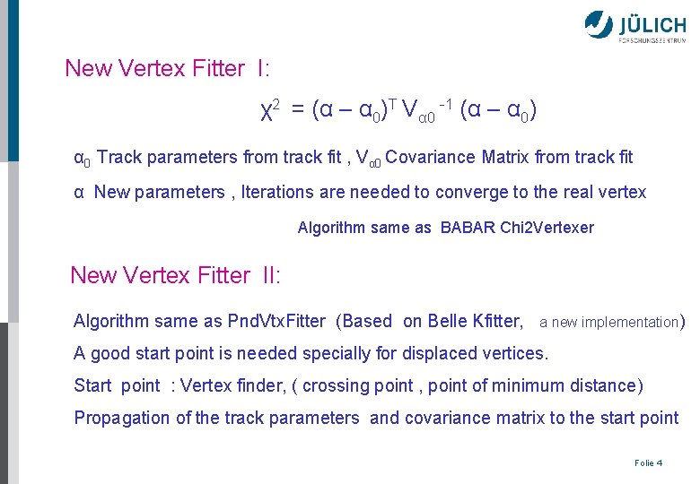
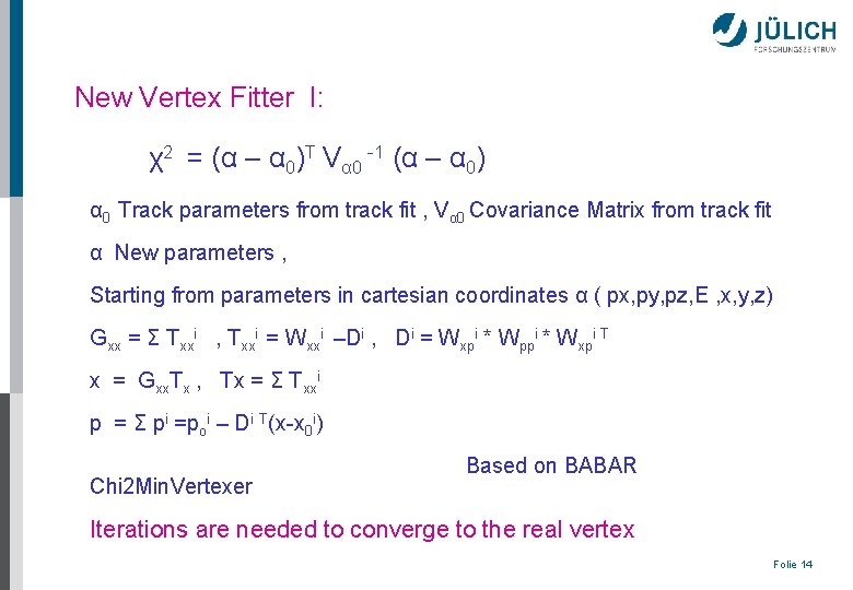
New Vertex Fitter I: χ2 = (α – α 0)T Vα 0 -1 (α – α 0) α 0 Track parameters from track fit , Vα 0 Covariance Matrix from track fit α New parameters , Iterations are needed to converge to the real vertex Algorithm same as BABAR Chi 2 Vertexer New Vertex Fitter II: Algorithm same as Pnd. Vtx. Fitter (Based on Belle Kfitter, a new implementation) A good start point is needed specially for displaced vertices. Start point : Vertex finder, ( crossing point , point of minimum distance) Propagation of the track parameters and covariance matrix to the start point Folie 4

New Vertex Fitter II : Least Square minimization with lagrange multiplier for constraints. χ2 = (α – α 0)T Vα 0 -1 (α – α 0)+ λ(D (α – αa )+ E(x – xa ) + d) The constraint equation H(α) =0 is linearized around suitable point (αa , xa ) D is derivative w. r. t α, E is derivative w. r. t x, d is H (αa , xa ) Minimize χ2 with respect to α , x and λ to determine track parameters and vertex Constraint : Tracks pass through an unknown point, For a solenoid field this leads to two constraints Folie 5

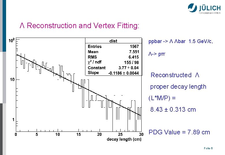
Λ Reconstruction and Vertex Fitting: ppbar -> Λ Λbar 1. 5 Ge. V/c, Λ-> pπ- Reconstructed Λ proper decay length (L*M/P) = 8. 43 ± 0. 313 cm PDG Value = 7. 89 cm Folie 6

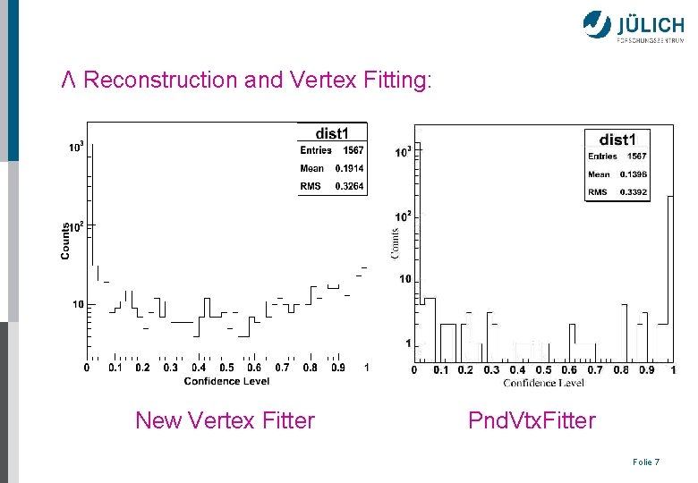
Λ Reconstruction and Vertex Fitting: New Vertex Fitter Pnd. Vtx. Fitter Folie 7

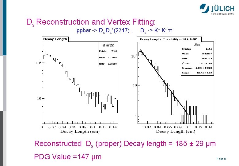
Ds Reconstruction and Vertex Fitting: ppbar -> Ds Ds*(2317) , Ds -> K+ K- π Reconstructed Ds (proper) Decay length = 185 ± 29 μm PDG Value =147 μm Folie 8

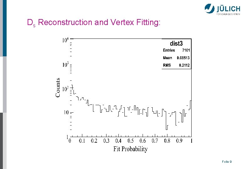
Ds Reconstruction and Vertex Fitting: Folie 9

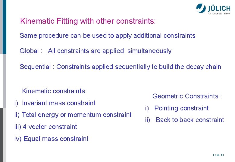
Kinematic Fitting with other constraints: Same procedure can be used to apply additional constraints Global : All constraints are applied simultaneously Sequential : Constraints applied sequentially to build the decay chain Kinematic constraints: i) Invariant mass constraint ii) Total energy or momentum constraint iii) 4 vector constraint Geometric Constraints : i) Pointing constraint ii) Back to back constraint iv) Equal mass constraint Folie 10

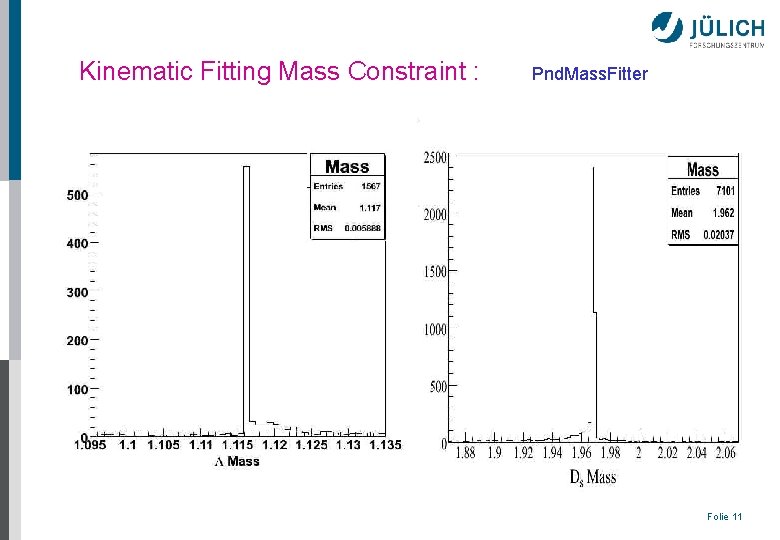
Kinematic Fitting Mass Constraint : Pnd. Mass. Fitter Folie 11

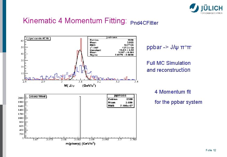
Kinematic 4 Momentum Fitting: Pnd 4 CFitter ppbar -> J/ψ π+πFull MC Simulation and reconstruction 4 Momentum fit for the ppbar system ) Folie 12

Summary and Outlook: New Vertex Fitters have been implemented Preliminary tests of its performance have been made. More detailed tests and improvements are in progress. Kinematic fitters with more constraints are planned to be included. Folie 13

New Vertex Fitter I: χ2 = (α – α 0)T Vα 0 -1 (α – α 0) α 0 Track parameters from track fit , Vα 0 Covariance Matrix from track fit α New parameters , Starting from parameters in cartesian coordinates α ( px, py, pz, E , x, y, z) Gxx = Σ Txxi , Txxi = Wxxi –Di , Di = Wxpi * Wppi * Wxpi T x = Gxx. Tx , Tx = Σ Txxi p = Σ pi =poi – Di T(x-x 0 i) Chi 2 Min. Vertexer Based on BABAR Iterations are needed to converge to the real vertex Folie 14