TEXTURE FEATURE EXTRACTION By Dr RAJEEV SRIVASTAVA IITBHU

TEXTURE FEATURE EXTRACTION By: Dr. RAJEEV SRIVASTAVA IIT(BHU), Varanasi

Definition: v Texture is repetition of patterns of local variation of pixel intensities. Texture feature is a measure method about relationship among the pixels in local area, reflecting the changes of image space gray levels. E. g.

Texture analysis: • There are three primary issues in texture analysis: Ø TEXTURE CLASSIFICATION Ø TEXTURE SEGMENTATION, and Ø SHAPE RECOVERY FROM TEXTURE.

v Texture classification: • In texture classification, the problem is identifying the given textured region from a given set of texture classes. • The texture analysis algorithms extract distinguishing feature from each region to facilitate classification of such patterns.

v Texture segmentation: • Unlike texture classification, texture segmentation is concerned with automatically determining the boundaries between various textured regions in an image. • Both reign-based methods and boundarybased methods have been attempted to segments texture images.

v Shape recovery from texture: • Image plane variation in the texture properties, such as density, size and orientation of texture primitives, are the cues exploited by shape – from-texture algorithms. • Quantifying the changes in the shape of texture elements is also useful to determine surface orientation.

TECHNIQUES FOR TEXTURE EXTRACTION • There are various techniques for texture extraction. Texture feature extraction algorithms can be grouped as follows: Ø Statistical Ø Geometrical Ø Model based Ø Signal Processing

v. Statistical method includes: A. Local features i. iii. iv. v. Grey level of central pixels, Average of grey levels in window, Median, Standard deviation of grey levels, Difference of maximum and minimum grey levels, vi. Difference between average grey level in small and large windows, vii. Kirsch feature, viii. Combine features

B. Galloway i. run length matrix C. Haralick i. co-occurrence matrix

v Geometrical method includes: Ø First threshold images into binary images of n grey levels. Ø Then calculate statistical features of connected areas.

v. Model based method includes: These involve building mathematical models to describe textures: ØMarkov random fields ØFractals 1 ØFractals 2

v Signal processing includes: These methods involve transforming original images using filters and calculating the energy of the transformed images. Ø Law’s masks Ø Laines – Daubechies wavelets Ø Fourier transform Ø Gabor filters

GRAY LEVEL CO-OCCURRENCE MATRIX

GRAY LEVEL CO-OCCURRENCE MATRIX Ø Also referred as co-occurrence distribution. Ø It is the most classical second-order statistical method for texture analysis. Ø An image is composed of pixels each with an intensity (a specific gray level), the GLCM is a tabulation of how often different combinations of gray levels co-occur in an image or image section.

Ø Texture feature calculations use the contents of the GLCM to give a measure of the variation in intensity at the pixel of interest. Ø GLCM texture feature operator produces a virtual variable which represents a specified texture calculation on a single beam echogram.

Steps for virtual variable creation: 1) Quantize the image data: Each sample on the echogram is treated as a single image pixel and its value is the intensity of that pixel. These intensities are then further quantized into a specified number of discrete gray levels, known as Quantization.

2. Create the GLCM: It will be a square matrix N in size where N is the Number of levels specified under Quantization. q Steps for matrix creation are: a) Let s be the sample under consideration for the calculation. b) Let W be the set of samples surrounding sample s which fall within a window centered upon sample s of the size specified under Window Size.

c) Define each element i, j of the GLCM of sample present in set W, as the number of times two samples of intensities i and j occur in specified Spatial relationship. d) The sum of all the elements i, j of the GLCM will be the total number of times the specified spatial relationship occurs in W.

e) Make the GLCM symmetric: i. Make a transposed copy of the GLCM. ii. Add this copy to the GLCM itself. • This produces a symmetric matrix in which the relationship i to j is indistinguishable for the relationship j to i. • Due to summation of all the elements i, j of the GLCM will now be twice the total number of times the specified spatial relationship occurs in W.

f) Normalize the GLCM: • Divide each element by the sum of all elements. • The elements of the GLCM may now be considered probabilities of finding the relationship i, j (or j, i) in W.

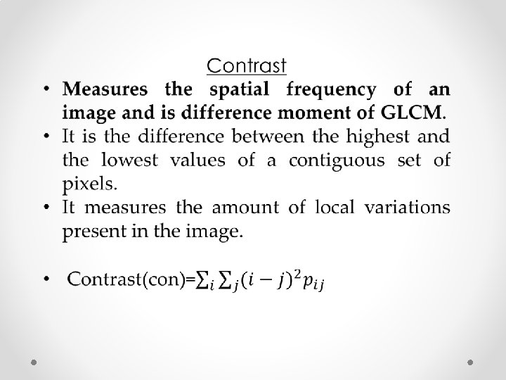
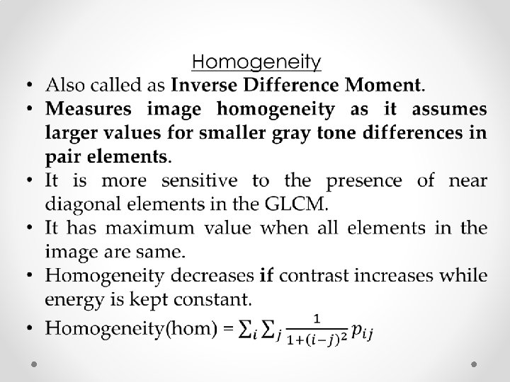
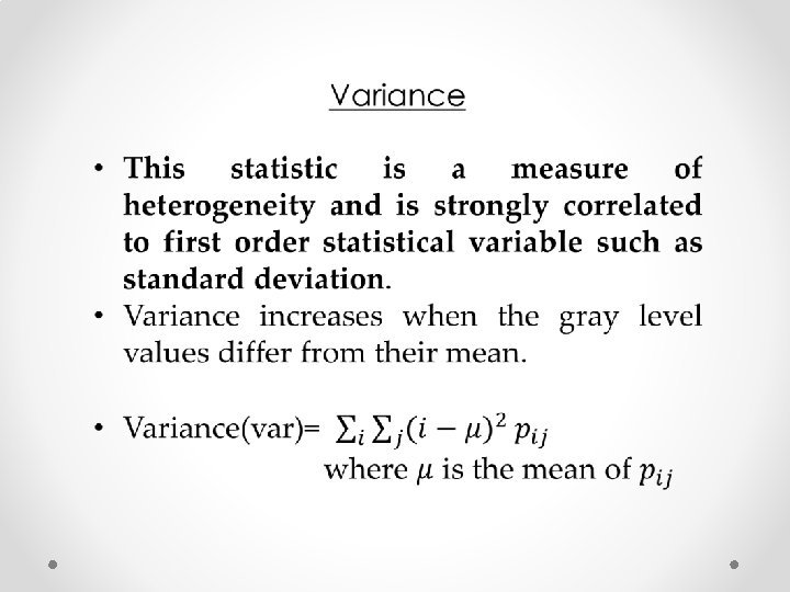
3) Calculate the selected Feature. This calculation uses only the values in the GLCM. For e. g. • Energy, • Entropy, • Contrast, • Homogeneity, • Correlation, • Shade or • Prominence 4) The sample s in the resulting virtual variable is replaced by the value of this calculated feature.

Framework for the GLCM: e. g. for glcm matrix for an image image 0 0 1 1 0 2 2 2 3 3 glcm matrix

Spatial relationship between two pixels: GLCM texture considers the relation between two pixels at a time, called the reference and the neighbor pixel 0 value -> ref pixel value: 1 2 3 0 0, 1 0, 2 0, 3 1 1, 0 1, 1 1, 2 1, 3 2 2, 0 2, 1 2, 2 2, 3 3 3, 0 3, 1 3, 2 3, 3 matrix framework

v In the above illustration, the neighbor pixel is chosen to be the one to the east (right) of each reference pixel. This can also be expressed as a (1, 0) relation: 1 pixel in the x direction, 0 pixels in the y direction.

v Each pixel within the window becomes the reference pixel in turn, starting in the upper left corner and proceeding to the lower right. Pixels along the right edge have no right hand neighbor, so they are not used for this count.

How to read the matrix framework: The top left cell will be filled with the number of times the combination 0, 0 occurs, i. e. how many times within the image area a pixel with grey level 0 (neighbor pixel) falls to the right of another pixel with grey level 0 (reference pixel).

How to read the east matrix: Twice in the test image the reference pixel is 0 and its eastern neighbor is also 0. Twice the reference pixel is 0 and its eastern neighbor is 1. Three times the reference pixel is 2 and its neighbor is also 2. 2 2 1 0 0 2 0 0 3 1 0 0 0 1 east matrix framework

UNDERSTANDING GLCM more: § GLCM represents the distance and angular spatial relationship over an image sub-region of specific size. § The GLCM calculates, how often a pixel with gray-level (grayscale intensity or Tone) value i occurs either horizontally, vertically, or diagonally to adjacent pixels with the value j.

GLCM directions of Analysis Ø Horizontal (0⁰) Ø Vertical (90⁰) Ø Diagonal: • Bottom left to top right (-45⁰) • Top left to bottom right (-135⁰) � � Denoted P₀, P₄₅, P₉₀, & P₁₃₅ Respectively. Ex. P₀ (i, j)

GLCM direction analysis:

v GLCM of an image is computed using a displacement vector d, defined by its radius δ and orientation θ. v Consider a 4 x 4 image represented by figure 1 a with four gray-tone values 0 through 3. A generalized GLCM for that image is shown in figure 1 b where #(i, j) stands for number of times i and j have been neighbors satisfying the condition stated by displacement vector d.

0 0 0 2 2 1 1 2 3 1 a. Test image 1 1 Gray tone 0 1 2 3 0 #(0, 0) #(0, 1) #(0, 2) #(0, 3) 1 #(1, 0) #(1, 1) #(1, 2) #(1, 3) 2 #(2, 0) #(2, 1) #(2, 2) #(2, 3) 3 #(3, 0) #(3, 1) #(3, 2) #(3, 3) 2 3 1 b. General form of GLCM

Ø The four GLCM for angles equal to 0°, 45°, 90° and 135° and radius equal to 1 are shown in figure 2 a-d.

4 2 1 0 6 0 2 4 0 0 0 4 2 0 1 0 6 1 2 2 0 0 1 2 0 0 2 0

4 1 0 0 2 1 3 0 1 2 2 0 1 2 1 0 0 2 4 1 3 1 0 2 0 0 1 0 0 0 2 0

v Choice of radius δ • δ values ranging should be ranging from 1, 2 to 10, but the best result is for δ = 1 and 2. • Applying large displacement value to a fine texture would yield a GLCM that does not capture detailed textural information. • As a pixel is more likely to be correlated to other closely located pixel than the one located far away, the above consideration is correct.

v Choice of angle θ • Every pixel has eight neighboring pixels allowing eight choices for θ, which are 0°, 45°, 90°, 135°, 180°, 225°, 270° or 315°. • According to the definition of GLCM, the cooccurring pairs obtained by choosing θ equal to 0° would be similar to those obtained by choosing θ equal to 180°. This concept extends to 0°, 45°, 90°and 135° as well. Hence, one has four choices to select the value of θ.

COMMON STATISTICS DERIVED FROM CO-OCCURRENCE PROBABILITIES

ENERGY • Also called Uniformity or Angular second moment. • Measures the textural uniformity that is pixel pair repetitions. • Detects disorders in textures. • Energy reaches a maximum value equal to one.

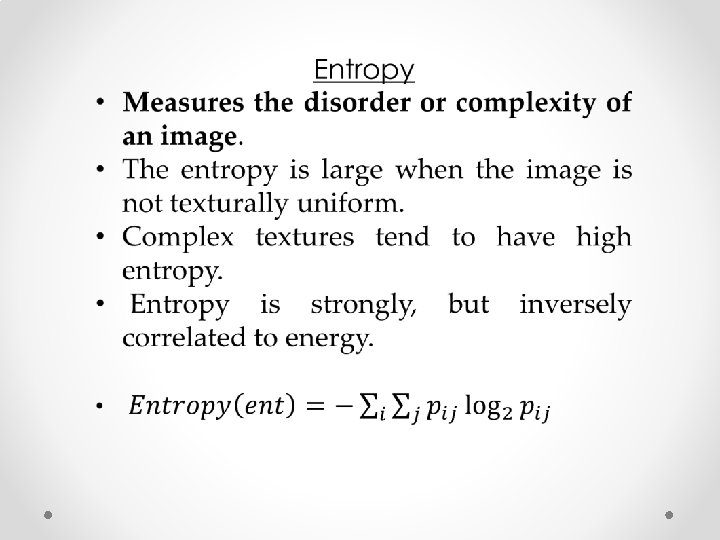
Difference Entropy

Gray level Difference Method

Gray level Difference Method • GLDM calculates the Gray level Difference Method Probability Density Functions for the given image. • This technique is usually used for extracting statistical texture features of a digital mammogram.

• The GLDM is based on the probability of occurrence that two pixels separated by a specific displacement vector 6 have a given difference. • The five textural features used in the experiments are contrast, angular second moment, entropy, mean, and inverse difference moment.

• In this study, we computed the probability density functions according to four kinds of displacement vectors and calculated textural features for each probability density function. • The four kinds of displacement vectors are considered, such as (0, d), (- d, d), (d, 0), (d, -d) where d is inter sample spacing distance.