Texture 1 Overview Introduction Painted textures Bump mapping
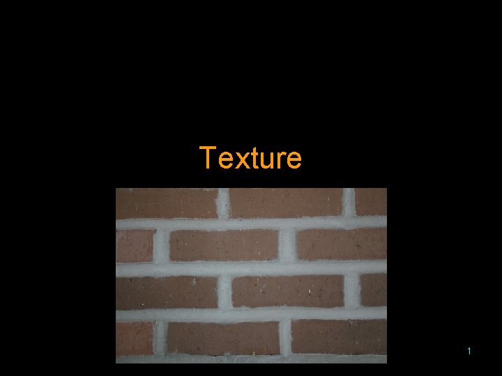
Texture 1
Overview • • Introduction Painted textures Bump mapping Environment mapping Three-dimensional textures Functional textures Antialiasing textures Open. GL details 2
Introduction • Few real objects are smooth • Textures can handle large repetitions – Brick wall – Stripes • Textures can handle small scale patterns – A brick’s roughness – Concrete – Wood grain • Textures are typically two dimensional images of what is being simulated 3

Painted Textures • A mapping of locations on the object into locations in the texture • The value from the texture replaces the diffuse component in the shading calculations • If the texture is larger than the object, only part of the texture is used or the texture is shrunk • If the object is larger than the texture, the texture is repeated across the object or the texture is stretched 4
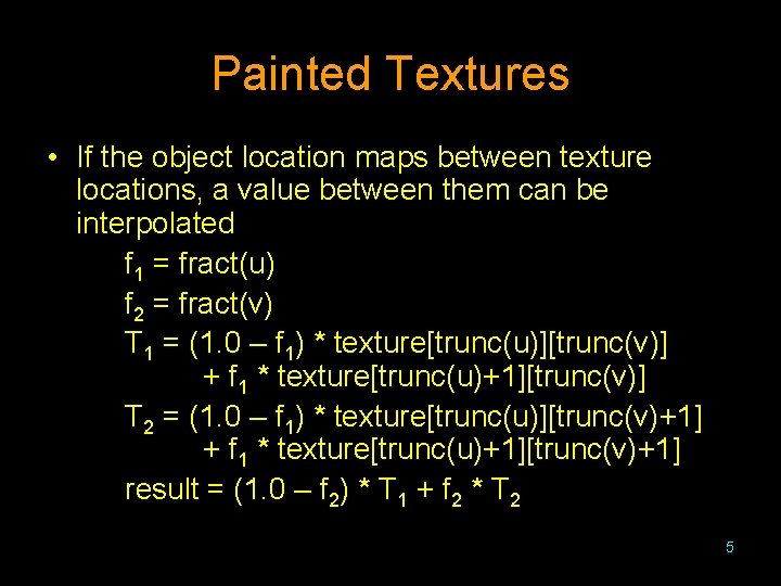
Painted Textures • If the object location maps between texture locations, a value between them can be interpolated f 1 = fract(u) f 2 = fract(v) T 1 = (1. 0 – f 1) * texture[trunc(u)][trunc(v)] + f 1 * texture[trunc(u)+1][trunc(v)] T 2 = (1. 0 – f 1) * texture[trunc(u)][trunc(v)+1] + f 1 * texture[trunc(u)+1][trunc(v)+1] result = (1. 0 – f 2) * T 1 + f 2 * T 2 5
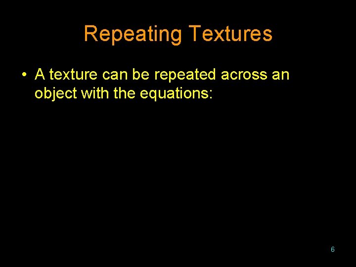
Repeating Textures • A texture can be repeated across an object with the equations: 6
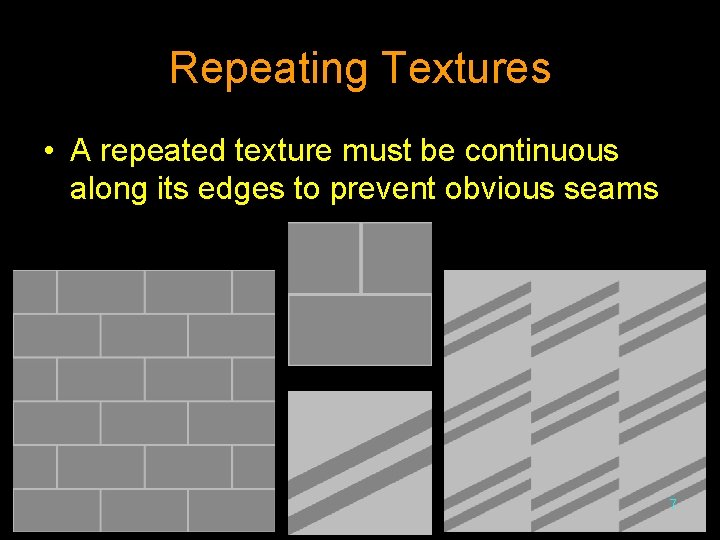
Repeating Textures • A repeated texture must be continuous along its edges to prevent obvious seams 7
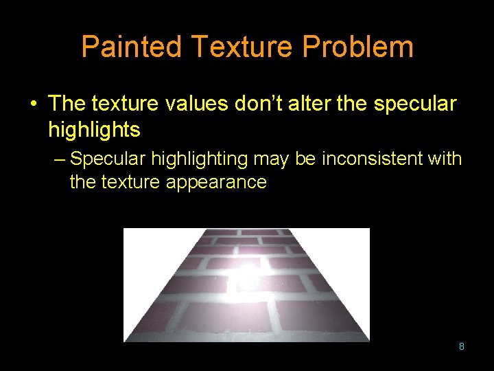
Painted Texture Problem • The texture values don’t alter the specular highlights – Specular highlighting may be inconsistent with the texture appearance 8

Bump Mapping • For a real bump, the surface normal changes when moving across the bump • A similar appearance can be created if a similar change is made to the surface normal for a plane 9
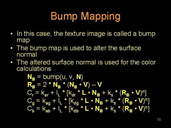
Bump Mapping • In this case, the texture image is called a bump map • The bump map is used to alter the surface normal • The altered surface normal is used for the color calculations NB = bump(u, v, N) RB = 2 * NB * (NB • V) – V Cr = kar + IL * [kdr * L • NB + ks * (RB • V)n] Cg = kag + IL * [kdg * L • NB + ks * (RB • V)n] Cb = kab + IL * [kdb * L • NB + ks * (RB • V)n] 10
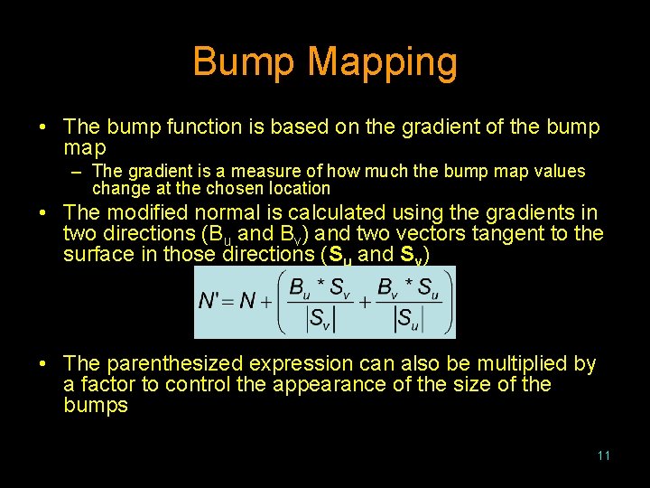
Bump Mapping • The bump function is based on the gradient of the bump map – The gradient is a measure of how much the bump map values change at the chosen location • The modified normal is calculated using the gradients in two directions (Bu and Bv) and two vectors tangent to the surface in those directions (Su and Sv) • The parenthesized expression can also be multiplied by a factor to control the appearance of the size of the bumps 11

Bump Mapping Examples • For the examples, the bump map is based on the product of the sine taken of the two coordinates: sin(10*u*π/1024) *sin(10*v*π/1024) 12

Bump Mapping Examples • A bump mapped plane using factors of 1. 0, 0. 5, and 2. 0 13

Bump Mapping Problem • Because the surface shape is not changed, “bumps” near the silhouette will not change the silhouette shape • If a bump mapped object is rotated, bumps will disappear when they reach the object profile 14
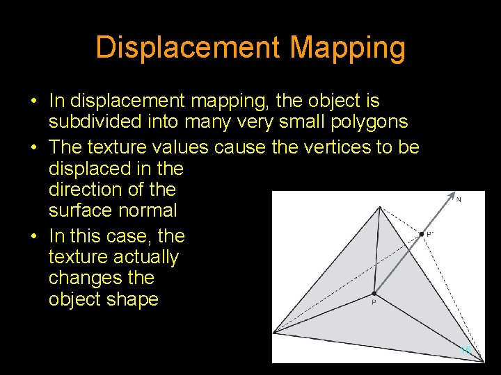
Displacement Mapping • In displacement mapping, the object is subdivided into many very small polygons • The texture values cause the vertices to be displaced in the direction of the surface normal • In this case, the texture actually changes the object shape 15
Environment Mapping • Environment mapping simulates reflective objects • An environment map is a rendering of the scene from inside the reflective object • The environment map is used to determine what would be seen in the reflection direction 16

Environment Mapping • The environment map can either be spherical or cube shaped – Spherical environment maps require a calculation to convert the direction through the sphere into a twodimensional matrix location 17
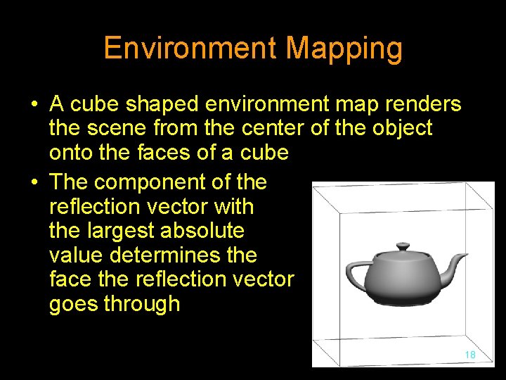
Environment Mapping • A cube shaped environment map renders the scene from the center of the object onto the faces of a cube • The component of the reflection vector with the largest absolute value determines the face the reflection vector goes through 18

Environment Mapping 19
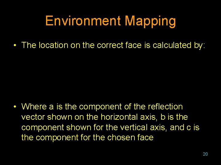
Environment Mapping • The location on the correct face is calculated by: • Where a is the component of the reflection vector shown on the horizontal axis, b is the component shown for the vertical axis, and c is the component for the chosen face 20
Three-Dimensional Textures • It is very difficult if not impossible to create a texture that can be wrapped around any irregularly shaped object without a visible discontinuity • Where a two-dimensional texture is applied to the surface, an object can be thought to be carved out of a three-dimensional texture • The storage requirements for a threedimensional texture are extremely large • Thus, three-dimensional textures are closely related to functional textures 21
Functional Textures • Instead of using a stored image as a texture, a functional texture uses a calculation based on the texture location • Because the function will be continuous in every direction, the texture is continuous in every direction • Instead of requiring space, these functional textures require computation time • By changing how the texture is calculated, many different textures can be created 22
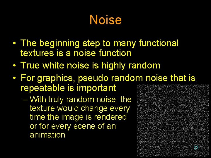
Noise • The beginning step to many functional textures is a noise function • True white noise is highly random • For graphics, pseudo random noise that is repeatable is important – With truly random noise, the texture would change every time the image is rendered or for every scene of an animation 23
Perlin Noise • Perlin developed a noise function this is used in many Hollywood movies • This noise function has: – No statistical variance when rotated – No statistical variance when translated – A narrow range of values 24
Turbulence • Typically the second step in functional textures is to build a turbulence function on top of the noise function • The functional textures are then built on top of the turbulence function • The turbulence function takes multiple samples of the noise function at many different frequencies • Different researchers will frequently develop their own turbulence function 25
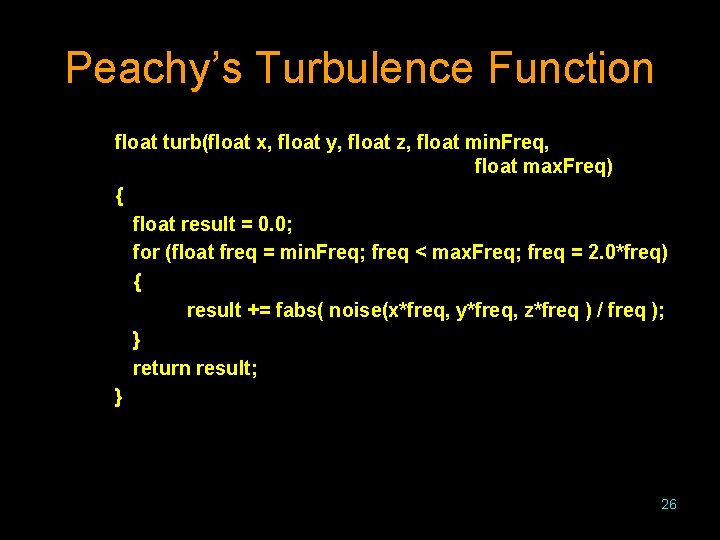
Peachy’s Turbulence Function float turb(float x, float y, float z, float min. Freq, float max. Freq) { float result = 0. 0; for (float freq = min. Freq; freq < max. Freq; freq = 2. 0*freq) { result += fabs( noise(x*freq, y*freq, z*freq ) / freq ); } return result; } 26
![Peachy’s Turbulence Results • These samples have frequency ranges of [1. 0, 4. 0], Peachy’s Turbulence Results • These samples have frequency ranges of [1. 0, 4. 0],](http://slidetodoc.com/presentation_image/a130af7abdeb7a39bdd4b743631a24ef/image-27.jpg)
Peachy’s Turbulence Results • These samples have frequency ranges of [1. 0, 4. 0], [1. 0, 16. 0], and [1. 0, 256. 0] 27
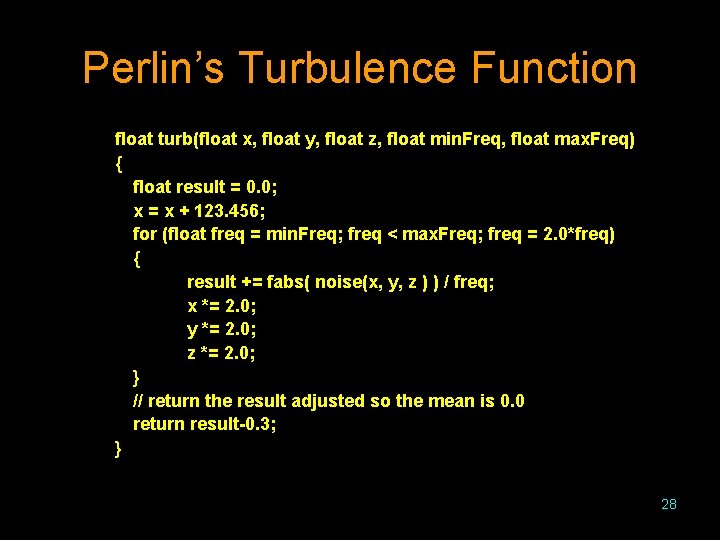
Perlin’s Turbulence Function float turb(float x, float y, float z, float min. Freq, float max. Freq) { float result = 0. 0; x = x + 123. 456; for (float freq = min. Freq; freq < max. Freq; freq = 2. 0*freq) { result += fabs( noise(x, y, z ) ) / freq; x *= 2. 0; y *= 2. 0; z *= 2. 0; } // return the result adjusted so the mean is 0. 0 return result-0. 3; } 28
![Perlin’s Turbulence Results • These samples have frequency ranges of [1. 0, 4. 0], Perlin’s Turbulence Results • These samples have frequency ranges of [1. 0, 4. 0],](http://slidetodoc.com/presentation_image/a130af7abdeb7a39bdd4b743631a24ef/image-29.jpg)
Perlin’s Turbulence Results • These samples have frequency ranges of [1. 0, 4. 0], [1. 0, 16. 0], and [1. 0, 256. 0] 29
Marble Texture • The Perlin/Ebert marble function uses a turbulence value to determine a color for the location void marble(float x, float y, float z, float color[3]) { float value = x + 3. 0 * turb(x, y, z, min. Freq, max. Freq); marble. Color( sin(π * value), color ); } • There are variations in how the marble. Color function is implemented – Linear interpolation between a light and dark color – Spline based interpolation between a light and dark color 30
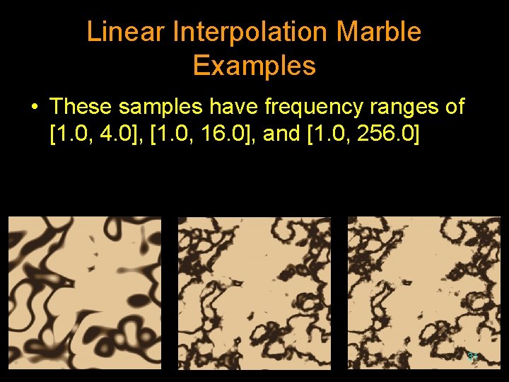
Linear Interpolation Marble Examples • These samples have frequency ranges of [1. 0, 4. 0], [1. 0, 16. 0], and [1. 0, 256. 0] 31
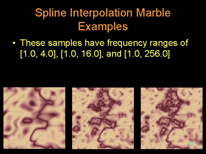
Spline Interpolation Marble Examples • These samples have frequency ranges of [1. 0, 4. 0], [1. 0, 16. 0], and [1. 0, 256. 0] 32
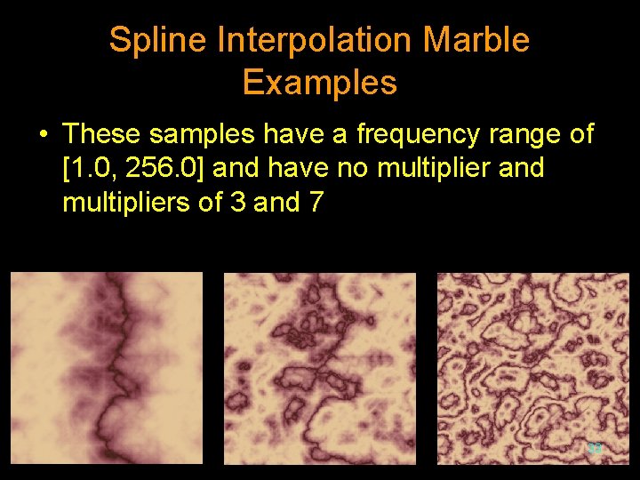
Spline Interpolation Marble Examples • These samples have a frequency range of [1. 0, 256. 0] and have no multiplier and multipliers of 3 and 7 33
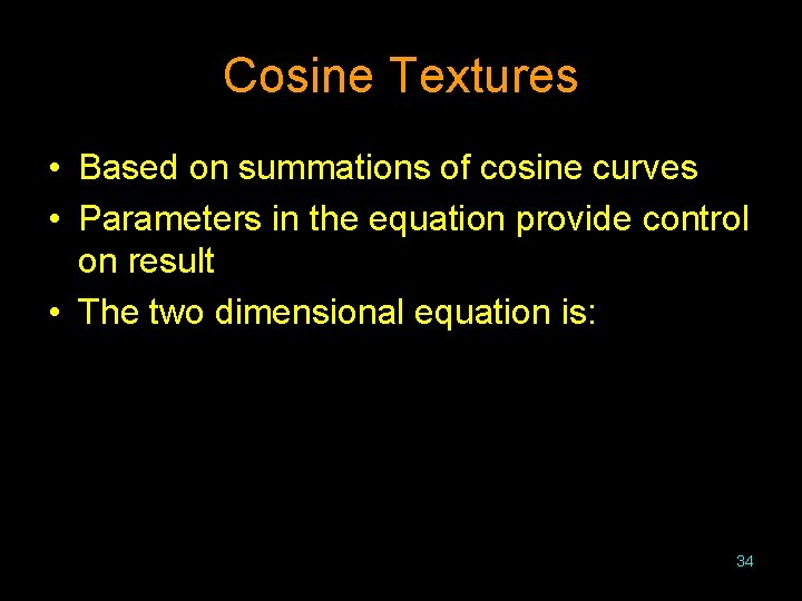
Cosine Textures • Based on summations of cosine curves • Parameters in the equation provide control on result • The two dimensional equation is: 34
Cosine Texture Parameters • The value of N controls the number of cosine terms – Typically between 4 and 7 • The constants ΦGx ΦGy are global phase shifts that move the pattern • The Ci terms change the amplitude of the various cosine components • The A 0 terms shift the pattern but are related to the Ci terms • The ωx 1 and ωy 1 determine the number of times the pattern repeats • The x and yi are phase values that are interdependent i with the base periods of x and y 35
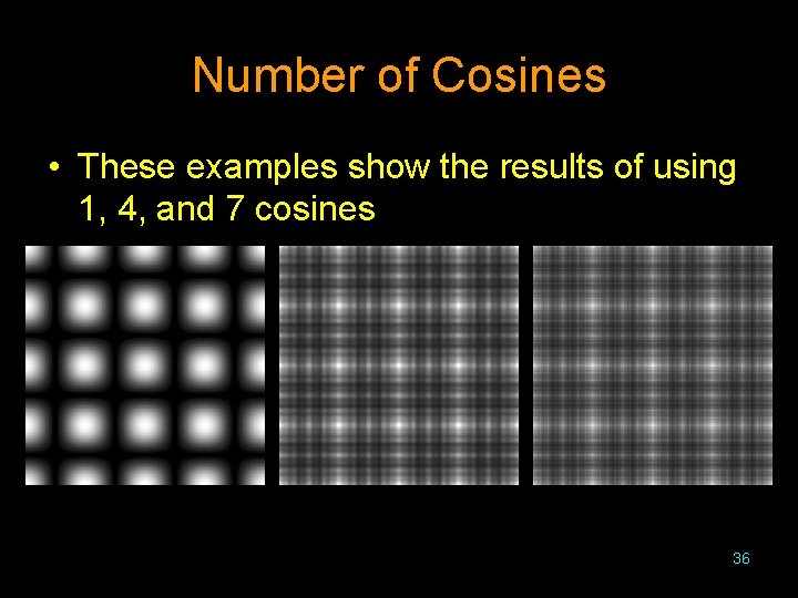
Number of Cosines • These examples show the results of using 1, 4, and 7 cosines 36
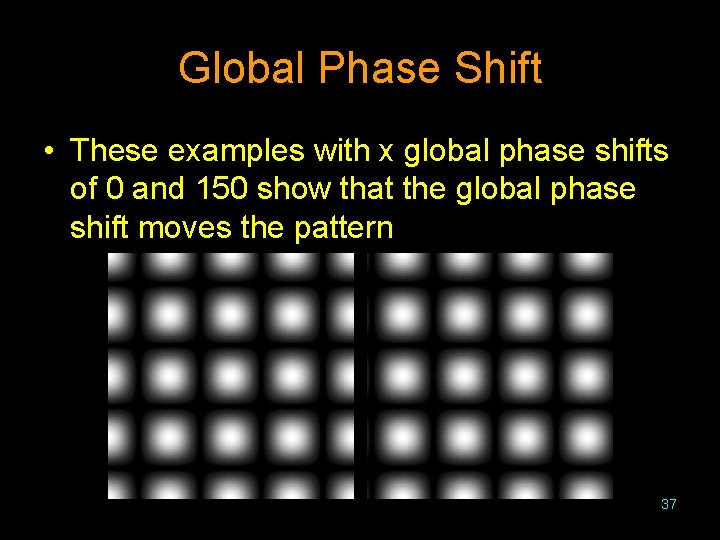
Global Phase Shift • These examples with x global phase shifts of 0 and 150 show that the global phase shift moves the pattern 37
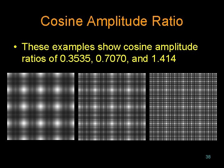
Cosine Amplitude Ratio • These examples show cosine amplitude ratios of 0. 3535, 0. 7070, and 1. 414 38
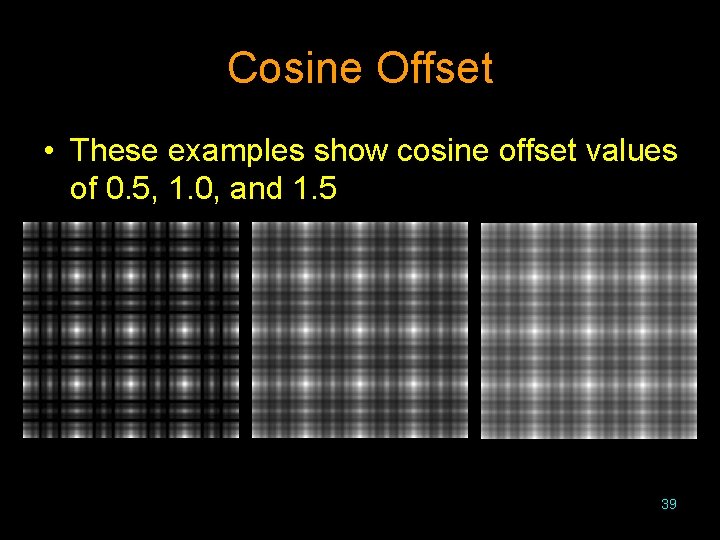
Cosine Offset • These examples show cosine offset values of 0. 5, 1. 0, and 1. 5 39
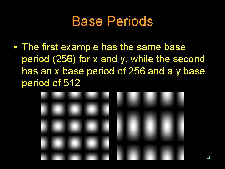
Base Periods • The first example has the same base period (256) for x and y, while the second has an x base period of 256 and a y base period of 512 40
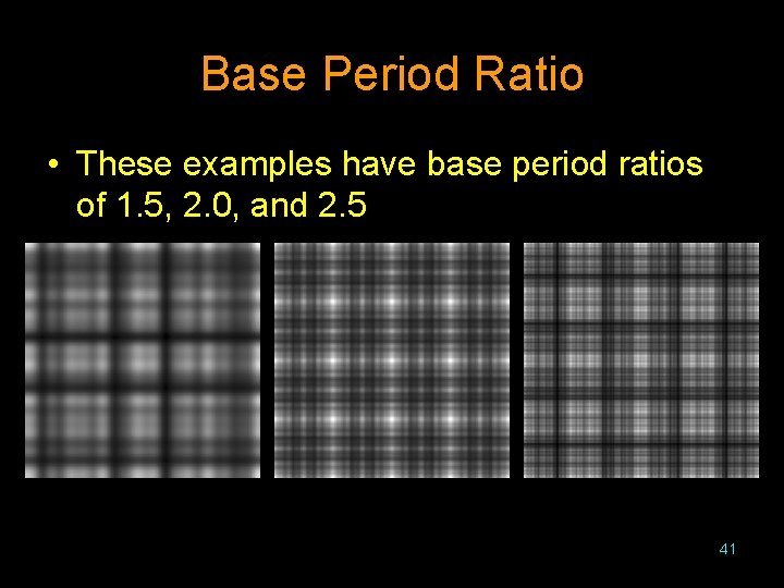
Base Period Ratio • These examples have base period ratios of 1. 5, 2. 0, and 2. 5 41
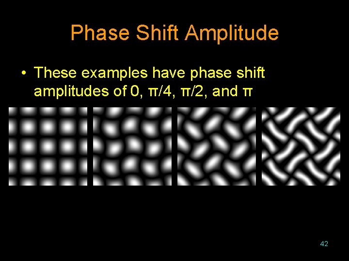
Phase Shift Amplitude • These examples have phase shift amplitudes of 0, π/4, π/2, and π 42
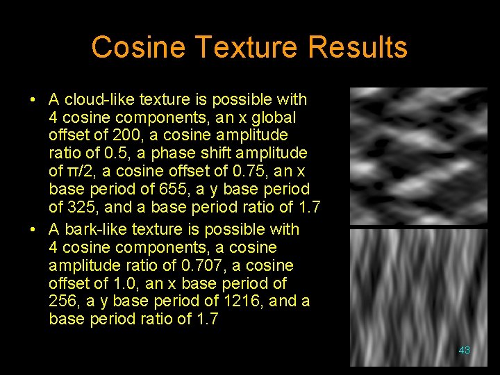
Cosine Texture Results • A cloud-like texture is possible with 4 cosine components, an x global offset of 200, a cosine amplitude ratio of 0. 5, a phase shift amplitude of π/2, a cosine offset of 0. 75, an x base period of 655, a y base period of 325, and a base period ratio of 1. 7 • A bark-like texture is possible with 4 cosine components, a cosine amplitude ratio of 0. 707, a cosine offset of 1. 0, an x base period of 256, a y base period of 1216, and a base period ratio of 1. 7 43
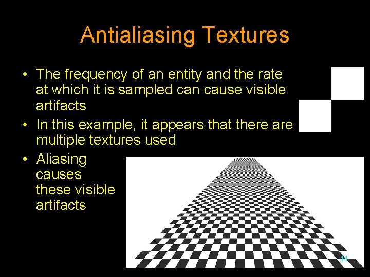
Antialiasing Textures • The frequency of an entity and the rate at which it is sampled can cause visible artifacts • In this example, it appears that there are multiple textures used • Aliasing causes these visible artifacts 44
Aliasing Corrections • Aliasing artifacts can be reduced by altering the sampling method • Common techniques include – Supersampling with jittering – Inverse mapping • Though the techniques are discussed relative to textures, they apply to other antialiasing applications 45
Supersampling • Multiple evenly spaced samples are taken from the texture for each location • An average or weighted average is taken of these samples to produce the final result • One weighted average uses 9 samples and the filter (weighting): 1 2 1 4 2 2 1 46
Supersampling With Jittering • Instead of taking evenly spaced samples, the sample locations are each shifted by a random amount • This helps to disturb a regular sampling frequency 47
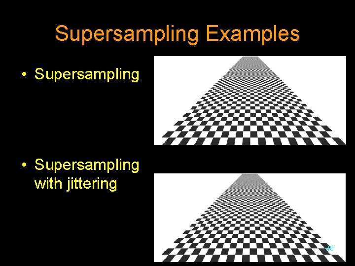
Supersampling Examples • Supersampling with jittering 48
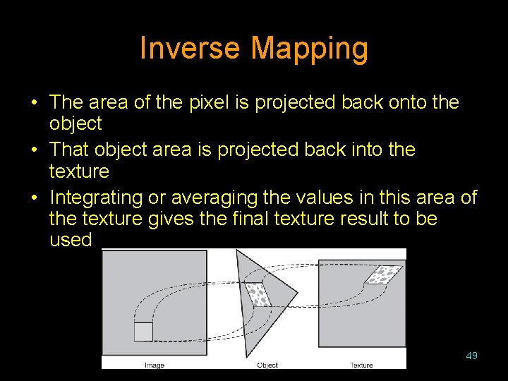
Inverse Mapping • The area of the pixel is projected back onto the object • That object area is projected back into the texture • Integrating or averaging the values in this area of the texture gives the final texture result to be used 49
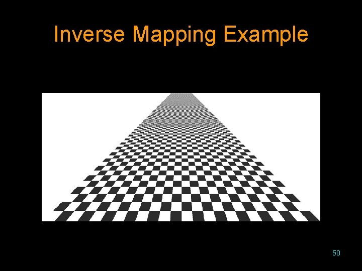
Inverse Mapping Example 50
Open. GL Texture • The steps to using texture in Open. GL are: – – Create or load the texture into Open. GL Enable texturing Specify how the texture is to be used Specify texture coordinates for polygon vertices or surface corners • Open. GL allows the programmer to specify if texture is to be added before or after the specular highlight • Open. GL allows textures of varying resolutions to deal with aliasing problems • Open. GL also has support for environment mapping 51
Texture Coordinates • The texture coordinates influence how the texture is applied • Texture coordinates are in the range [0. 0, 1. 0] • If Open. GL is told to repeat the texture, values outside of this range cause multiple copies of the texture to be used • If Open. GL is told to clamp the coordinates, any values below the range will be set to 0. 0 and any above the range will be set to 1. 0 52
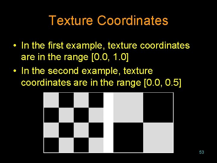
Texture Coordinates • In the first example, texture coordinates are in the range [0. 0, 1. 0] • In the second example, texture coordinates are in the range [0. 0, 0. 5] 53
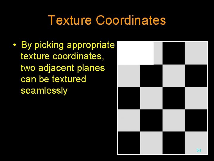
Texture Coordinates • By picking appropriate texture coordinates, two adjacent planes can be textured seamlessly 54
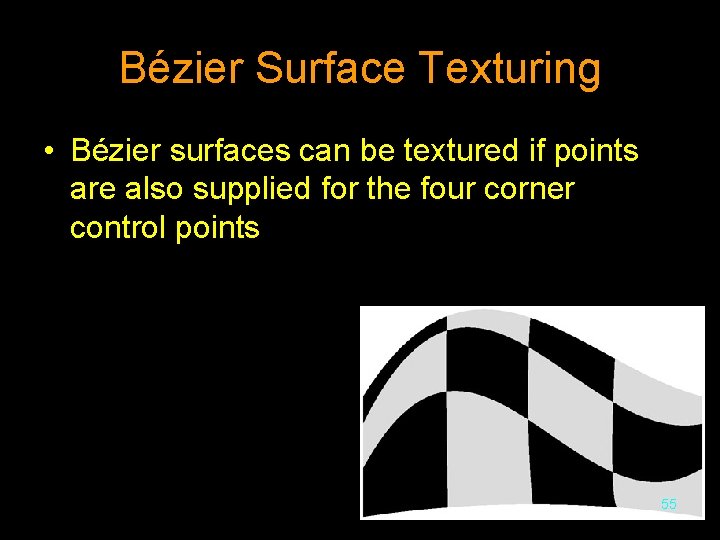
Bézier Surface Texturing • Bézier surfaces can be textured if points are also supplied for the four corner control points 55
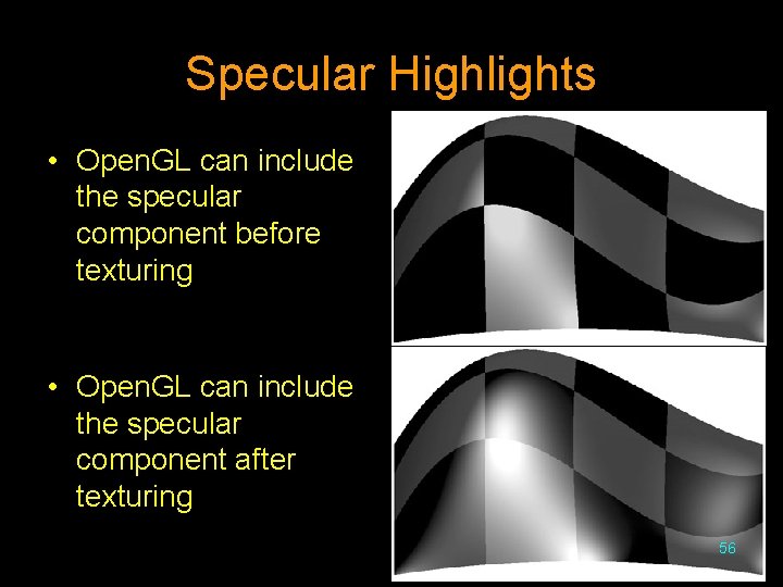
Specular Highlights • Open. GL can include the specular component before texturing • Open. GL can include the specular component after texturing 56
- Slides: 56