Textbook for the Statistical Parametric Mapping SPM class

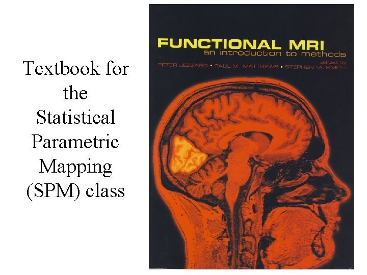
Textbook for the Statistical Parametric Mapping (SPM) class

Statistical Parametric Mapping Chapter 3 Principles of Nuclear Magnetic Resonance and MRI Many thanks to those that share their MRI slides online

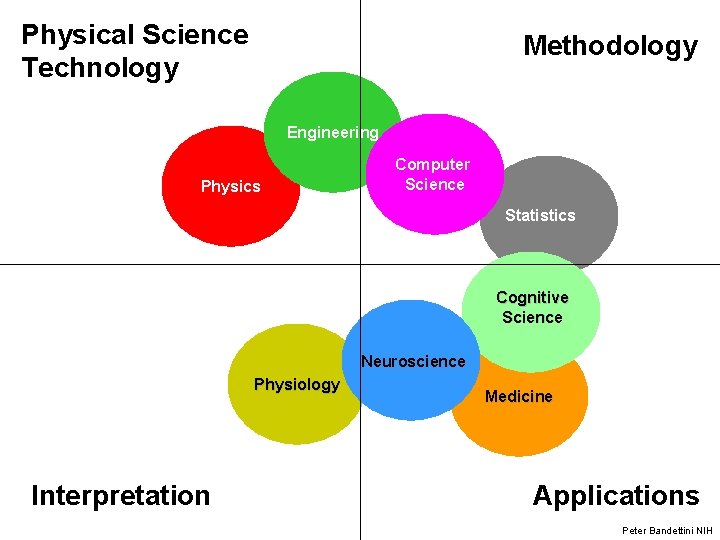
Physical Science Technology Methodology Engineering Physics Computer Science Statistics Cognitive Science Neuroscience Physiology Interpretation Medicine Applications Peter Bandettini NIH

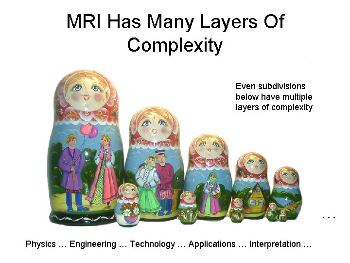
MRI Has Many Layers Of Complexity Even subdivisions below have multiple layers of complexity … Physics … Engineering … Technology … Applications … Interpretation …

History: MRI • 1940 s – Bloch & Purcell: Nuclear Magnetic Resonance • 1973 - Lauterbur: gradients for spatial localization of images • 1977 – Mansfield: first image of human anatomy, first echo planar image (a fast imaging technique) • 1990 s - Discovery that MRI can be used to distinguish oxygenated blood from deoxygenated blood. Leads to Functional Magnetic Resonance imaging (f. MRI) • Paul Lauterbur and Peter Mansfield won the Nobel Prize in Physiology/Medicine (2003) for their pioneering work in MRI

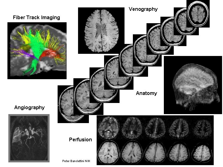
Venography Fiber Track Imaging Anatomy Angiography Perfusion Peter Bandettini NIH

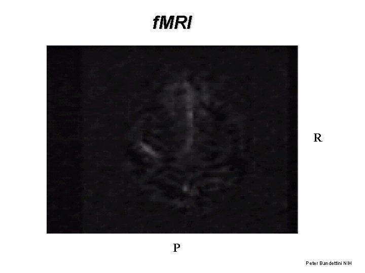
f. MRI R P Peter Bandettini NIH

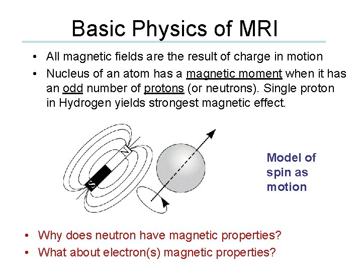
Basic Physics of MRI • All magnetic fields are the result of charge in motion • Nucleus of an atom has a magnetic moment when it has an odd number of protons (or neutrons). Single proton in Hydrogen yields strongest magnetic effect. Model of spin as motion • Why does neutron have magnetic properties? • What about electron(s) magnetic properties?

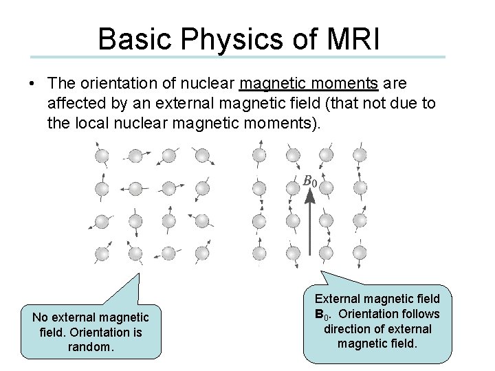
Basic Physics of MRI • The orientation of nuclear magnetic moments are affected by an external magnetic field (that not due to the local nuclear magnetic moments). No external magnetic field. Orientation is random. External magnetic field B 0. Orientation follows direction of external magnetic field.

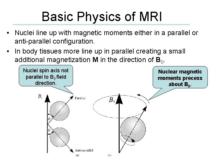
Basic Physics of MRI • Nuclei line up with magnetic moments either in a parallel or anti-parallel configuration. • In body tissues more line up in parallel creating a small additional magnetization M in the direction of B 0. Nuclei spin axis not parallel to B 0 field direction. Nuclear magnetic moments precess about B 0.

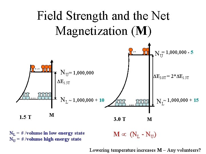
Field Strength and the Net Magnetization (M). . . NU= 1, 000 - 5 NU = 1, 000 ΔE 3. 0 T = 2*ΔE 1. 5 T . . . 1. 5 T NL ~ 1, 000 + 10 M NL = # /volume in low energy state NU = # /volume high energy state NL~ 1, 000 + 15 . . . 3. 0 T M M (NL - NU) Lowering temperature increases M – Any volunteers?

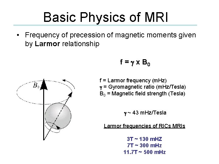
Basic Physics of MRI • Frequency of precession of magnetic moments given by Larmor relationship f = g x B 0 f = Larmor frequency (m. Hz) g = Gyromagnetic ratio (m. Hz/Tesla) B 0 = Magnetic field strength (Tesla) g ~ 43 m. Hz/Tesla Larmor frequencies of RICs MRIs 3 T ~ 130 m. HZ 7 T ~ 300 m. Hz 11. 7 T ~ 500 m. Hz

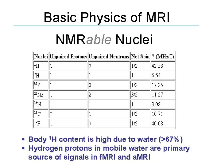
Basic Physics of MRI NMRable Nuclei § Body 1 H content is high due to water (>67%) § Hydrogen protons in mobile water are primary source of signals in f. MRI and a. MRI

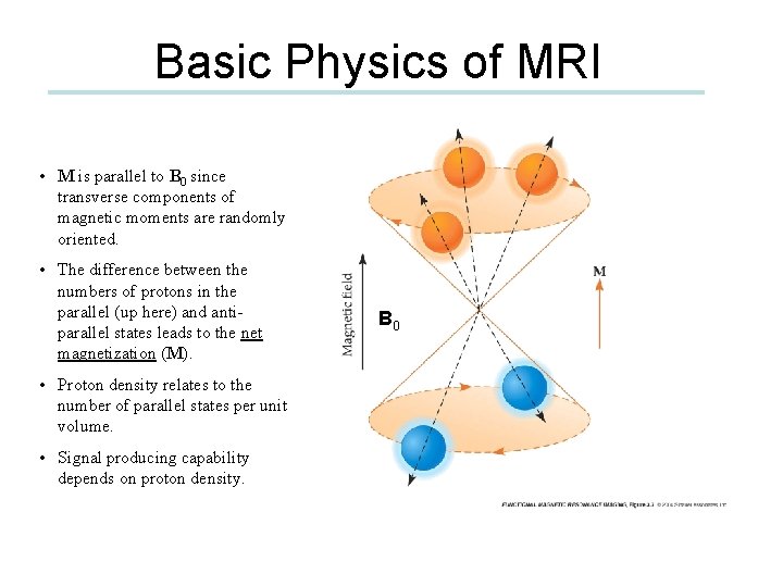
Basic Physics of MRI • M is parallel to B 0 since transverse components of magnetic moments are randomly oriented. • The difference between the numbers of protons in the parallel (up here) and antiparallel states leads to the net magnetization (M). • Proton density relates to the number of parallel states per unit volume. • Signal producing capability depends on proton density. B 0

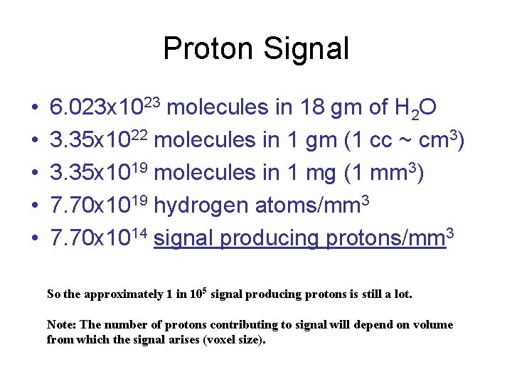
Proton Signal • • • 6. 023 x 1023 molecules in 18 gm of H 2 O 3. 35 x 1022 molecules in 1 gm (1 cc ~ cm 3) 3. 35 x 1019 molecules in 1 mg (1 mm 3) 7. 70 x 1019 hydrogen atoms/mm 3 7. 70 x 1014 signal producing protons/mm 3 So the approximately 1 in 105 signal producing protons is still a lot. Note: The number of protons contributing to signal will depend on volume from which the signal arises (voxel size).

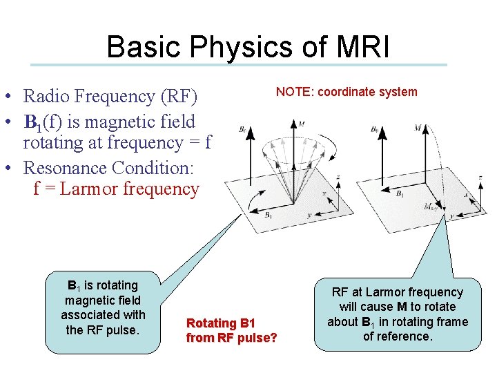
Basic Physics of MRI • Radio Frequency (RF) • B 1(f) is magnetic field rotating at frequency = f • Resonance Condition: f = Larmor frequency B 1 is rotating magnetic field associated with the RF pulse. NOTE: coordinate system Rotating B 1 from RF pulse? RF at Larmor frequency will cause M to rotate about B 1 in rotating frame of reference.

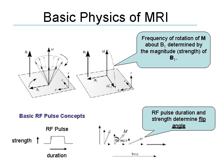
Basic Physics of MRI Frequency of rotation of M about B 1 determined by the magnitude (strength) of B 1. Basic RF Pulse Concepts RF Pulse strength duration RF pulse duration and strength determine flip angle

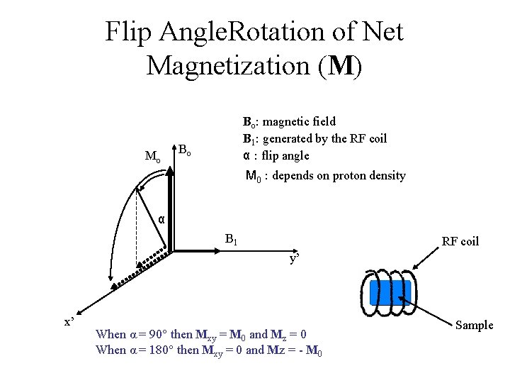
Flip Angle. Rotation of Net Magnetization (M) Mo Bo: magnetic field B 1: generated by the RF coil α : flip angle Bo M 0 : depends on proton density α B 1 RF coil y’ x’ When α = 90° then Mxy = M 0 and Mz = 0 When α = 180° then Mxy = 0 and Mz = - M 0 Sample

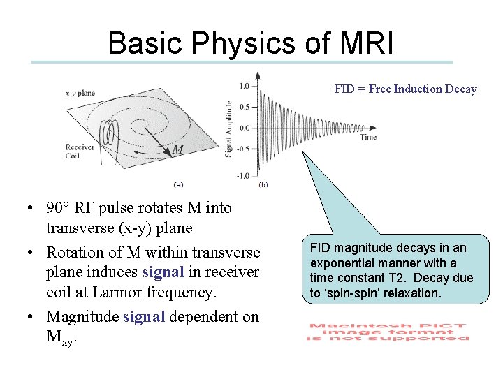
Basic Physics of MRI FID = Free Induction Decay • 90° RF pulse rotates M into transverse (x-y) plane • Rotation of M within transverse plane induces signal in receiver coil at Larmor frequency. • Magnitude signal dependent on Mxy. FID magnitude decays in an exponential manner with a time constant T 2. Decay due to ‘spin-spin’ relaxation.

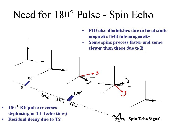
Need for 180° Pulse - Spin Echo • FID also diminishes due to local static magnetic field inhomogeneity • Some spins precess faster and some slower than those due to B 0 90° 0 tim e 180° TE/2 - • 180 ° RF pulse reverses dephasing at TE (echo time) • Residual decay due to T 2 TE/2 + TE Spin Echo Signal

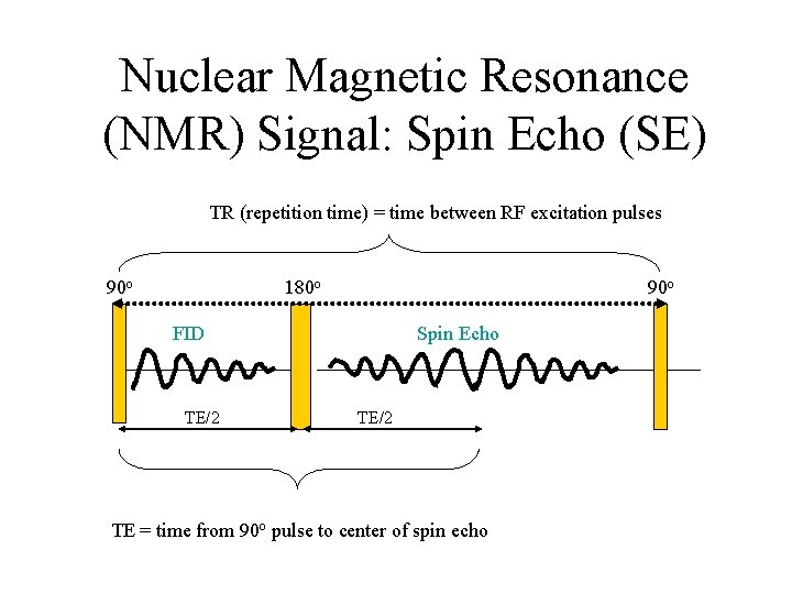
Nuclear Magnetic Resonance (NMR) Signal: Spin Echo (SE) TR (repetition time) = time between RF excitation pulses 90 o 180 o FID TE/2 Spin Echo TE/2 TE = time from 90 o pulse to center of spin echo

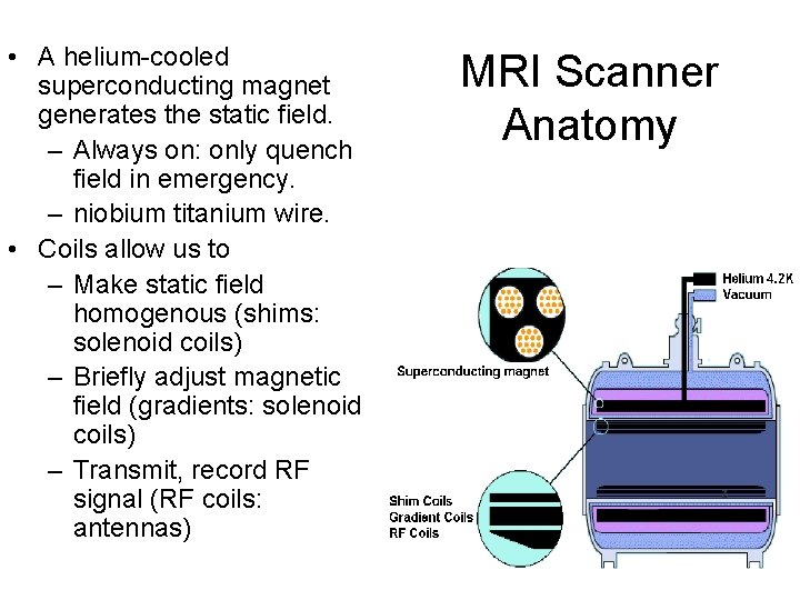
• A helium-cooled superconducting magnet generates the static field. – Always on: only quench field in emergency. – niobium titanium wire. • Coils allow us to – Make static field homogenous (shims: solenoid coils) – Briefly adjust magnetic field (gradients: solenoid coils) – Transmit, record RF signal (RF coils: antennas) MRI Scanner Anatomy

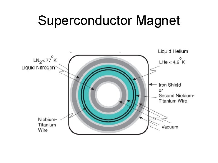
Superconductor Magnet

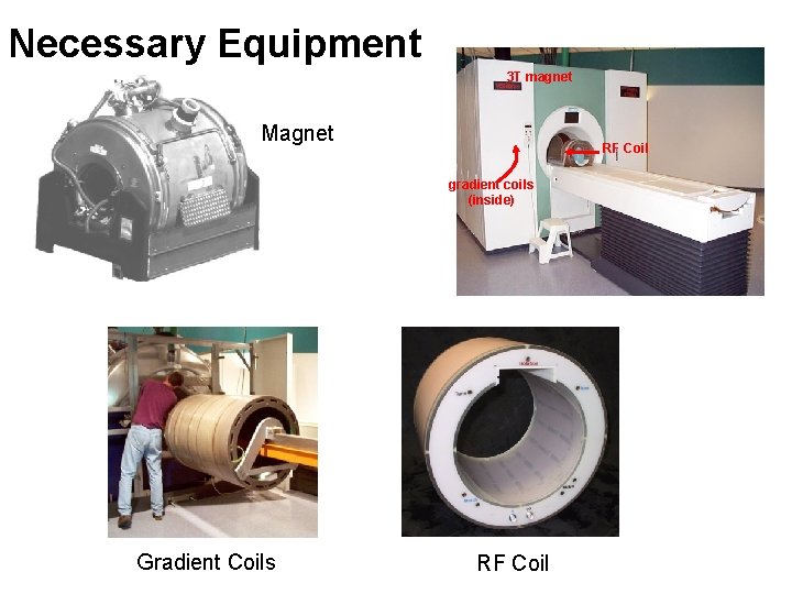
Necessary Equipment 3 T magnet Magnet RF Coil gradient coils (inside) Gradient Coils RF Coil

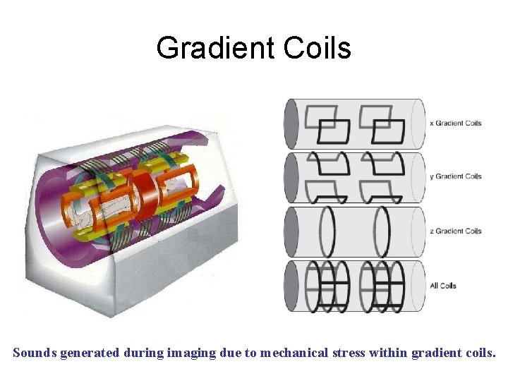
Gradient Coils Sounds generated during imaging due to mechanical stress within gradient coils.

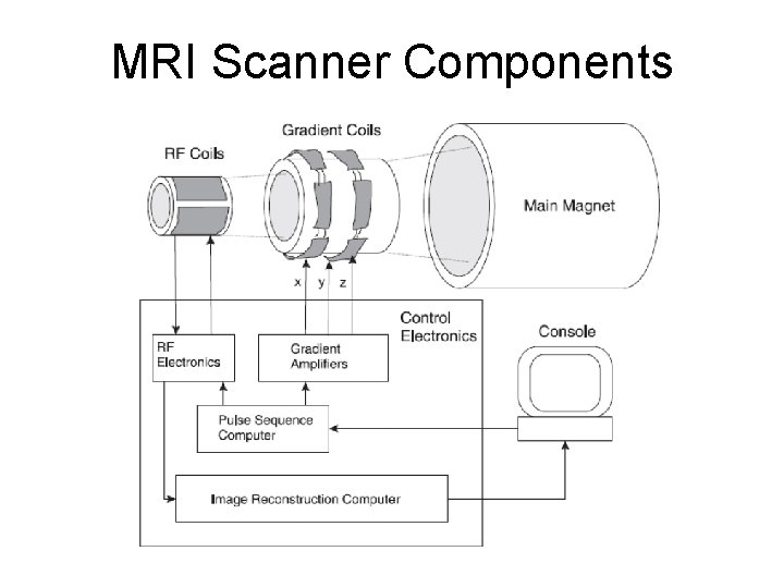
MRI Scanner Components

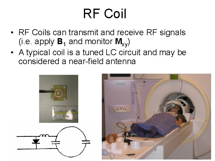
RF Coil • RF Coils can transmit and receive RF signals (i. e. apply B 1 and monitor Mxy) • A typical coil is a tuned LC circuit and may be considered a near-field antenna

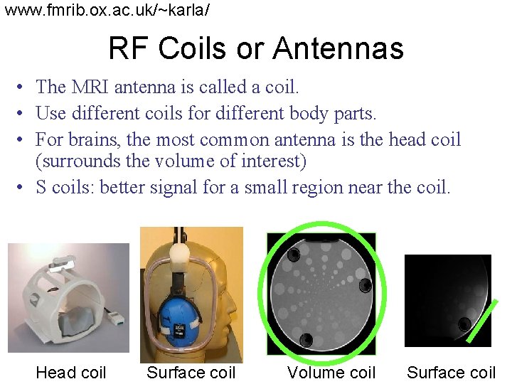
www. fmrib. ox. ac. uk/~karla/ RF Coils or Antennas • The MRI antenna is called a coil. • Use different coils for different body parts. • For brains, the most common antenna is the head coil (surrounds the volume of interest) • S coils: better signal for a small region near the coil. Head coil Surface coil Volume coil Surface coil

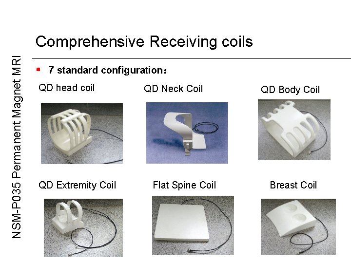
NSM-P 035 Permanent Magnet MRI Comprehensive Receiving coils § 7 standard configuration： QD head coil QD Extremity Coil QD Neck Coil Flat Spine Coil QD Body Coil Breast Coil

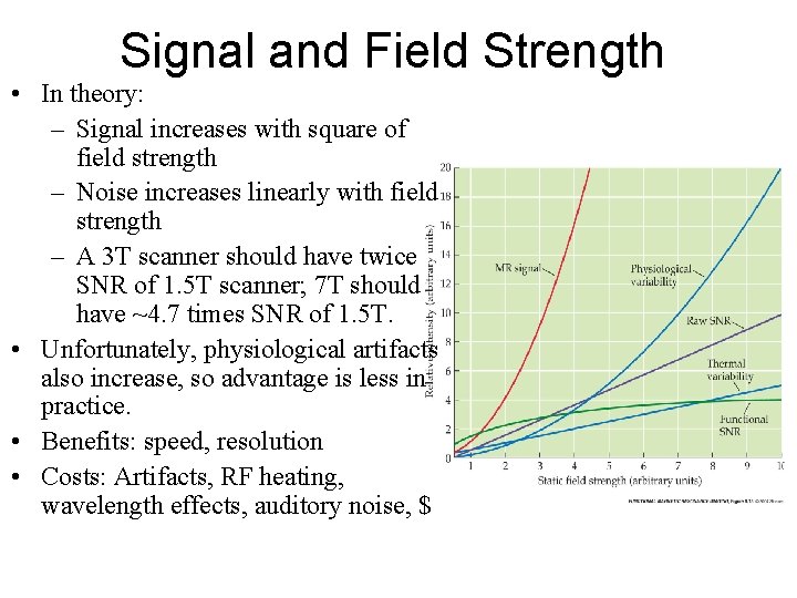
Signal and Field Strength • In theory: – Signal increases with square of field strength – Noise increases linearly with field strength – A 3 T scanner should have twice SNR of 1. 5 T scanner; 7 T should have ~4. 7 times SNR of 1. 5 T. • Unfortunately, physiological artifacts also increase, so advantage is less in practice. • Benefits: speed, resolution • Costs: Artifacts, RF heating, wavelength effects, auditory noise, $

Making Images of the NMR Signal • Uniform magnetic field to set the stage (Main Magnet) • Gradient coils for positional information • RF transceiver (excite and receive) • Digitizer (convert received analog to digital) • Pulse sequencer (controls timing of gradients, RF, and digitizer) • Computer (FFT to form images, store pulse sequences, display results, archive, etc. )

Role of Gradient Coils • Coils that produce magnetic field gradients along x-, y-, and z-directions to encode spatial information • Selective excitation: (during RF) excite those spins within a thin “slice” of the subject • Frequency encoding: (during readout) make the signal’s frequency depend on position • Phase encoding: (between excitation and Phase encoding readout) make the signal’s phase depend on position

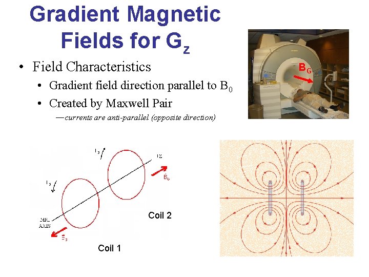
Gradient Magnetic Fields for Gz • Field Characteristics • Gradient field direction parallel to B 0 • Created by Maxwell Pair — currents are anti-parallel (opposite direction) Coil 2 Coil 1 BG

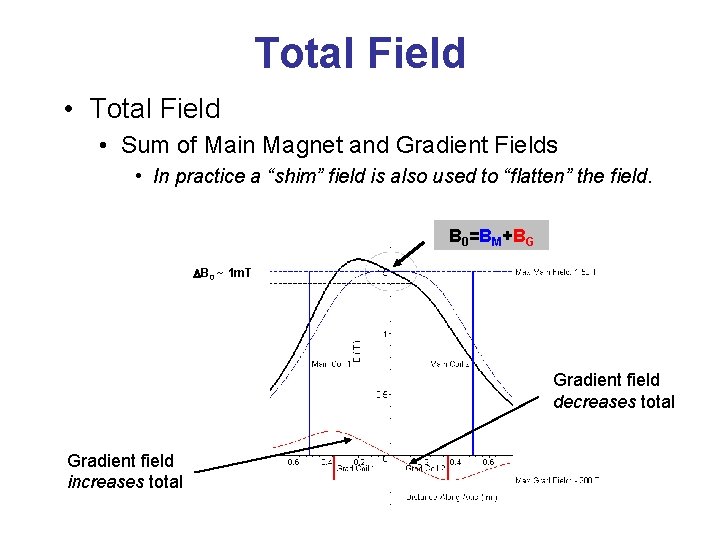
Total Field • Total Field • Sum of Main Magnet and Gradient Fields • In practice a “shim” field is also used to “flatten” the field. B 0=BM+BG DB 0 ~ 1 m. T Gradient field decreases total Gradient field increases total

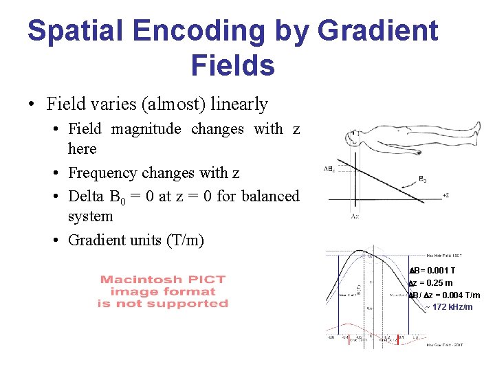
Spatial Encoding by Gradient Fields • Field varies (almost) linearly • Field magnitude changes with z here • Frequency changes with z • Delta B 0 = 0 at z = 0 for balanced system • Gradient units (T/m) DB= 0. 001 T Dz = 0. 25 m DB/ Dz = 0. 004 T/m ~ 172 k. Hz/m

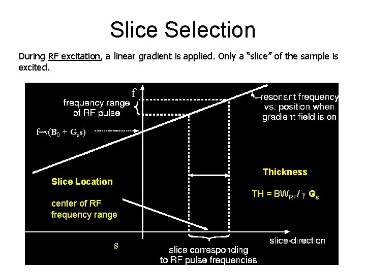
Slice Selection During RF excitation, a linear gradient is applied. Only a “slice” of the sample is excited. f f= (B 0 + Gss) Thickness Slice Location center of RF frequency range s TH = BWRF/ Gs

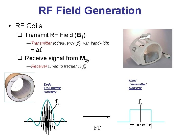
RF Field Generation • RF Coils q Transmit RF Field (B 1) — Transmitter at frequency f 0 with bandwidth = Df q Receive signal from Mxy — Receiver tuned to frequency f 0 Head Transmitter/ Receiver Body Transmitter/ Receiver fo t fo FT Df = 1/ t

Frequency encoding During signal readout, a gradient is applied in one direction: B(x) = B 0 + Gxx f(x) = {B 0 + Gxx} D f(x) = Gxx Mxy f(x) The precession frequency of the net magnetization Mxy depends on x-location. A Fourier transform of the time signal can determine where the nuclei are along the x-direction.

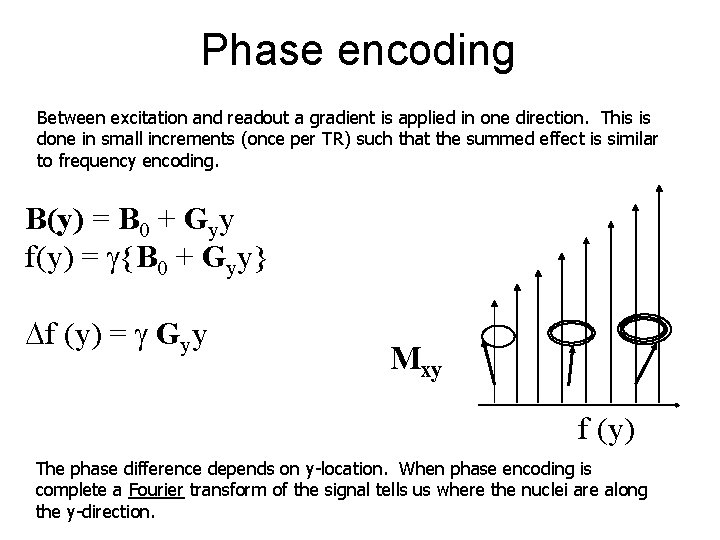
Phase encoding Between excitation and readout a gradient is applied in one direction. This is done in small increments (once per TR) such that the summed effect is similar to frequency encoding. B(y) = B 0 + Gyy f(y) = {B 0 + Gyy} Df (y) = Gyy Mxy f (y) The phase difference depends on y-location. When phase encoding is complete a Fourier transform of the signal tells us where the nuclei are along the y-direction.

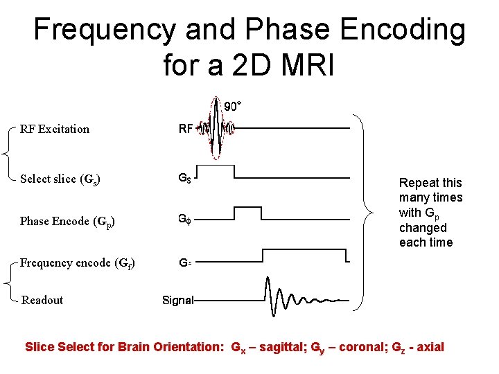
Frequency and Phase Encoding for a 2 D MRI RF Excitation Select slice (Gs) Phase Encode (Gp) Repeat this many times with Gp changed each time Frequency encode (Gf) Readout Slice Select for Brain Orientation: Gx – sagittal; Gy – coronal; Gz - axial

Making an Image k-space (frequency domain) A k-space domain image is formed using frequency and phase encoding

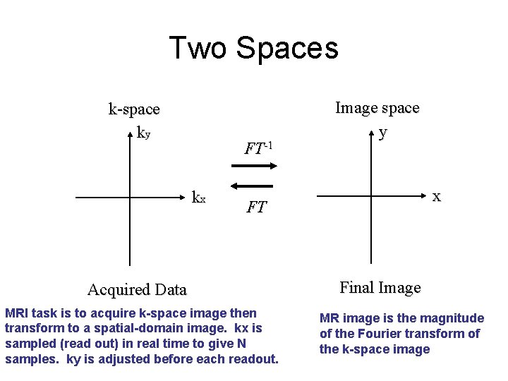
Two Spaces k-space ky FT-1 kx Image space y x FT Acquired Data MRI task is to acquire k-space image then transform to a spatial-domain image. kx is sampled (read out) in real time to give N samples. ky is adjusted before each readout. Final Image MR image is the magnitude of the Fourier transform of the k-space image

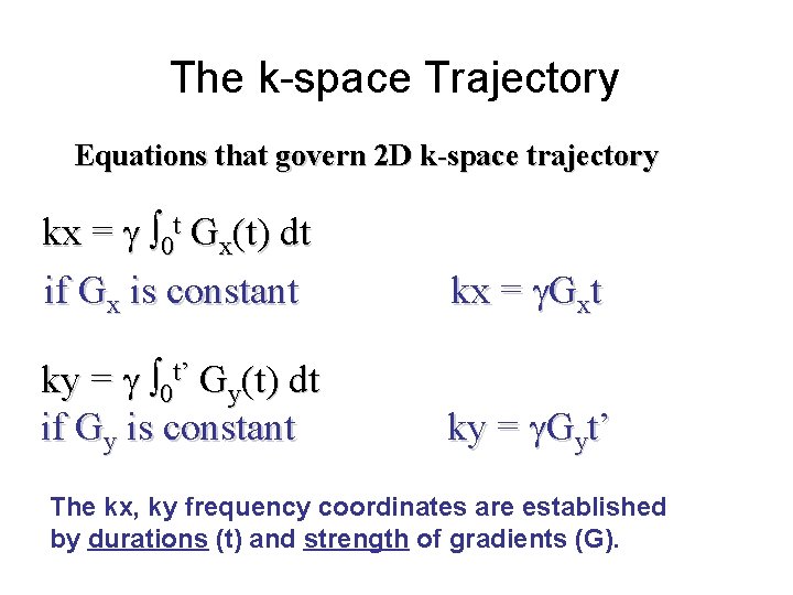
The k-space Trajectory Equations that govern 2 D k-space trajectory kx = 0 t Gx(t) dt if Gx is constant kx = Gxt ky = 0 t’ Gy(t) dt if Gy is constant ky = Gyt’ The kx, ky frequency coordinates are established by durations (t) and strength of gradients (G).

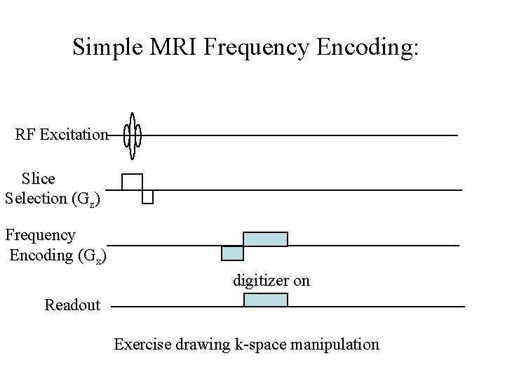
Simple MRI Frequency Encoding: RF Excitation Slice Selection (Gz) Frequency Encoding (Gx) digitizer on Readout Exercise drawing k-space manipulation

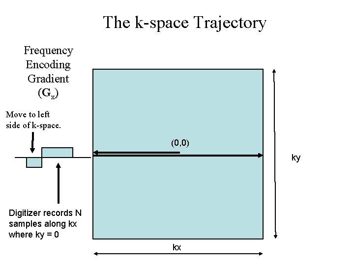
The k-space Trajectory Frequency Encoding Gradient (Gx) Move to left side of k-space. (0, 0) ky Digitizer records N samples along kx where ky = 0 kx

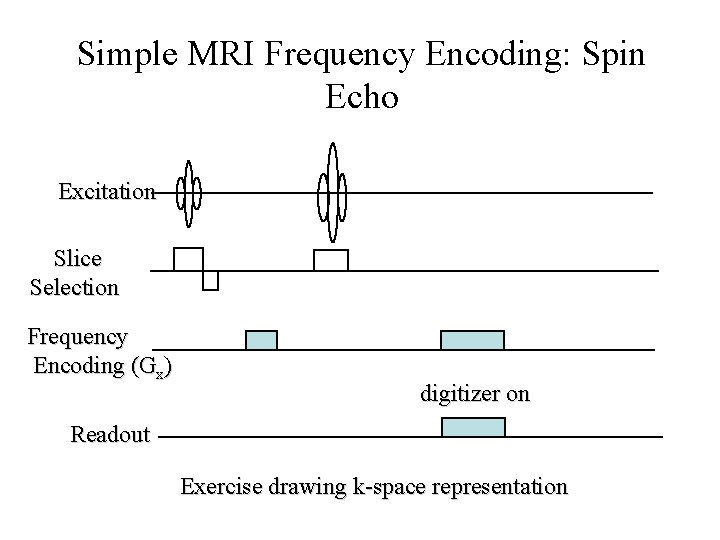
Simple MRI Frequency Encoding: Spin Echo Excitation Slice Selection Frequency Encoding (Gx) digitizer on Readout Exercise drawing k-space representation

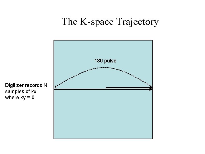
The K-space Trajectory 180 pulse Digitizer records N samples of kx where ky = 0

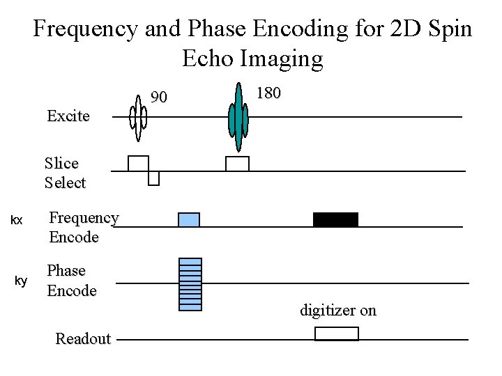
Frequency and Phase Encoding for 2 D Spin Echo Imaging Excite 90 180 Slice Select kx ky Frequency Encode Phase Encode digitizer on Readout

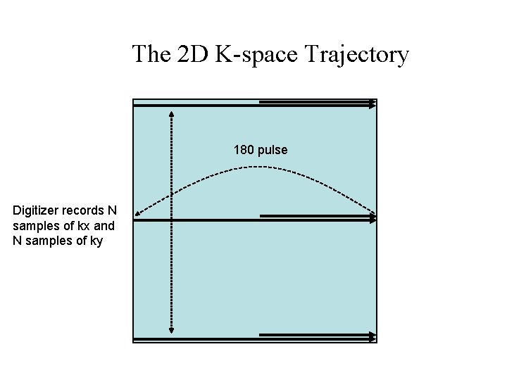
The 2 D K-space Trajectory 180 pulse Digitizer records N samples of kx and N samples of ky

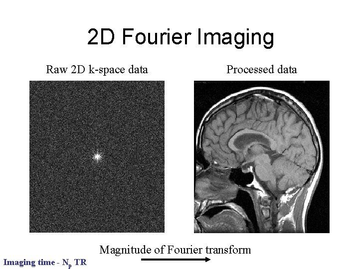
2 D Fourier Imaging Raw 2 D k-space data Processed data Magnitude of Fourier transform Imaging time - Np TR

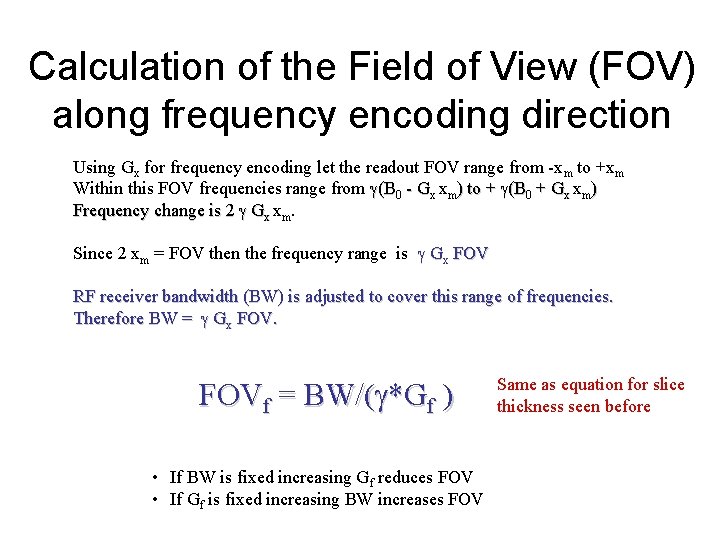
Calculation of the Field of View (FOV) along frequency encoding direction Using Gx for frequency encoding let the readout FOV range from -xm to +xm Within this FOV frequencies range from (B 0 - Gx xm) to + (B 0 + Gx xm) Frequency change is 2 Gx xm. Since 2 xm = FOV then the frequency range is Gx FOV RF receiver bandwidth (BW) is adjusted to cover this range of frequencies. Therefore BW = Gx FOVf = BW/( *Gf ) • If BW is fixed increasing Gf reduces FOV • If Gf is fixed increasing BW increases FOV Same as equation for slice thickness seen before

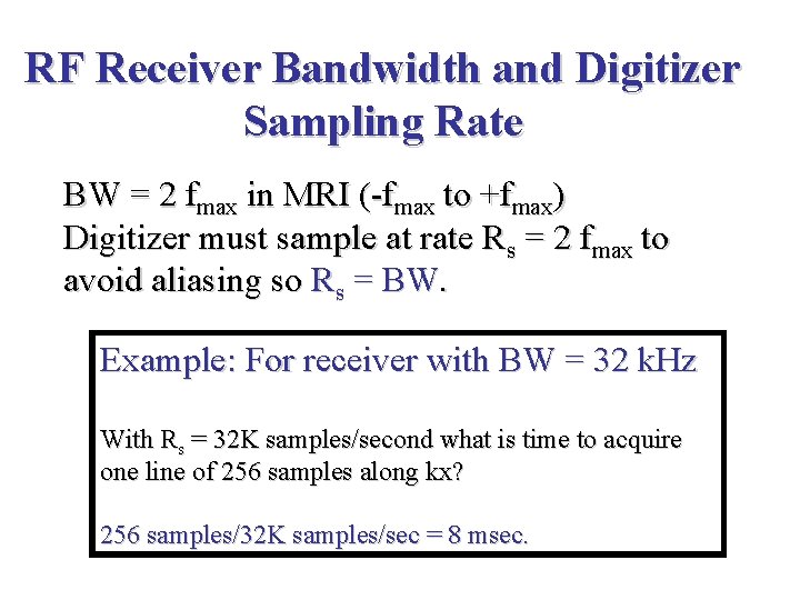
RF Receiver Bandwidth and Digitizer Sampling Rate BW = 2 fmax in MRI (-fmax to +fmax) Digitizer must sample at rate Rs = 2 fmax to avoid aliasing so Rs = BW. Example: For receiver with BW = 32 k. Hz With Rs = 32 K samples/second what is time to acquire one line of 256 samples along kx? 256 samples/32 K samples/sec = 8 msec.

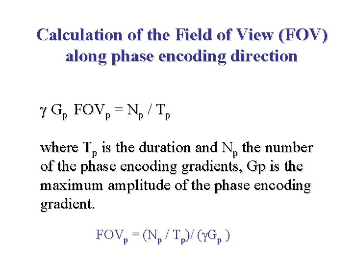
Calculation of the Field of View (FOV) along phase encoding direction Gp FOVp = Np / Tp where Tp is the duration and Np the number of the phase encoding gradients, Gp is the maximum amplitude of the phase encoding gradient. FOVp = (Np / Tp)/ ( Gp )

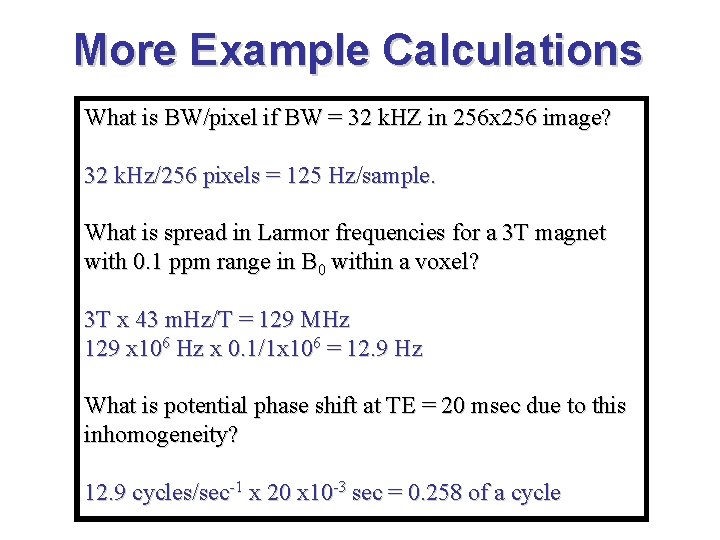
More Example Calculations What is BW/pixel if BW = 32 k. HZ in 256 x 256 image? 32 k. Hz/256 pixels = 125 Hz/sample. What is spread in Larmor frequencies for a 3 T magnet with 0. 1 ppm range in B 0 within a voxel? 3 T x 43 m. Hz/T = 129 MHz 129 x 106 Hz x 0. 1/1 x 106 = 12. 9 Hz What is potential phase shift at TE = 20 msec due to this inhomogeneity? 12. 9 cycles/sec-1 x 20 x 10 -3 sec = 0. 258 of a cycle

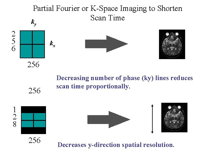
Partial Fourier or K-Space Imaging to Shorten Scan Time k y 2 5 6 kx 256 Decreasing number of phase (ky) lines reduces scan time proportionally. 1 2 8 256 Decreases y-direction spatial resolution.

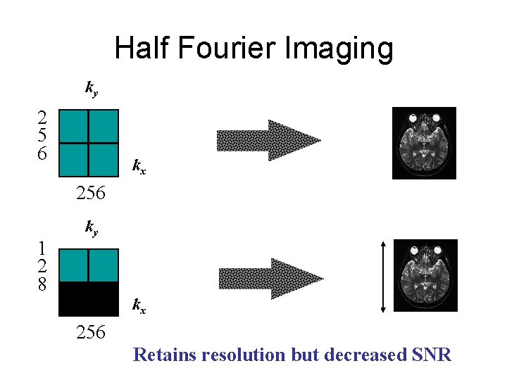
Half Fourier Imaging ky 2 5 6 kx 256 1 2 8 ky kx 256 Retains resolution but decreased SNR

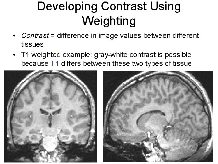
Developing Contrast Using Weighting • Contrast = difference in image values between different tissues • T 1 weighted example: gray-white contrast is possible because T 1 differs between these two types of tissue

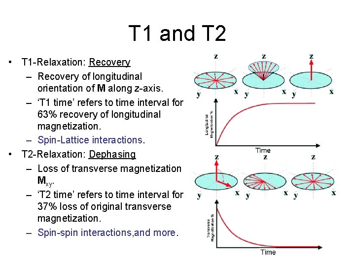
T 1 and T 2 • T 1 -Relaxation: Recovery – Recovery of longitudinal orientation of M along z-axis. – ‘T 1 time’ refers to time interval for 63% recovery of longitudinal magnetization. – Spin-Lattice interactions. • T 2 -Relaxation: Dephasing – Loss of transverse magnetization Mxy. – ‘T 2 time’ refers to time interval for 37% loss of original transverse magnetization. – Spin-spin interactions, and more.

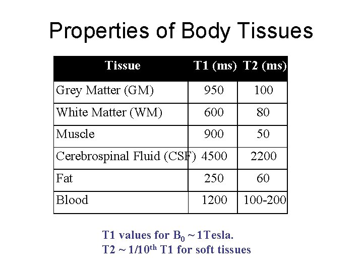
Properties of Body Tissues Tissue T 1 (ms) T 2 (ms) Grey Matter (GM) 950 100 White Matter (WM) 600 80 Muscle 900 50 Cerebrospinal Fluid (CSF) 4500 2200 Fat 250 60 Blood 1200 100 -200 T 1 values for B 0 ~ 1 Tesla. T 2 ~ 1/10 th T 1 for soft tissues

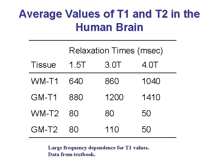
Average Values of T 1 and T 2 in the Human Brain Relaxation Times (msec) Tissue 1. 5 T 3. 0 T 4. 0 T WM-T 1 640 860 1040 GM-T 1 880 1200 1410 WM-T 2 80 80 50 GM-T 2 80 110 50 Large frequency dependence for T 1 values. Data from textbook.

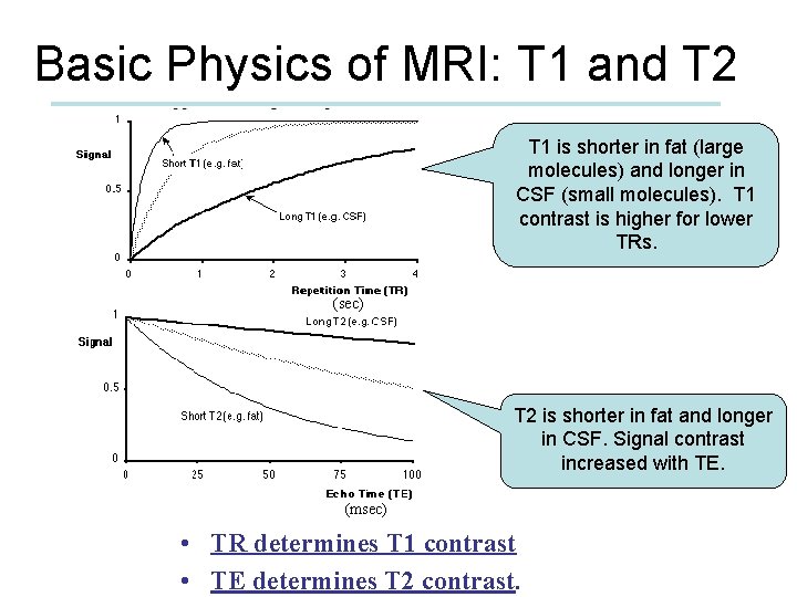
Basic Physics of MRI: T 1 and T 2 T 1 is shorter in fat (large molecules) and longer in CSF (small molecules). T 1 contrast is higher for lower TRs. (sec) T 2 is shorter in fat and longer in CSF. Signal contrast increased with TE. (msec) • TR determines T 1 contrast • TE determines T 2 contrast.

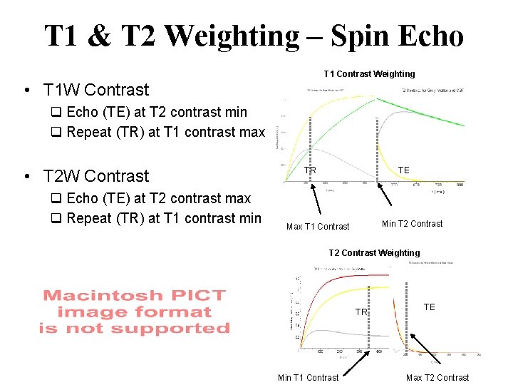
T 1 & T 2 Weighting – Spin Echo T 1 Contrast Weighting • T 1 W Contrast q Echo (TE) at T 2 contrast min q Repeat (TR) at T 1 contrast max • T 2 W Contrast q Echo (TE) at T 2 contrast max q Repeat (TR) at T 1 contrast min TR TE Min T 2 Contrast Max T 1 Contrast T 2 Contrast Weighting TR Min T 1 Contrast TE Max T 2 Contrast

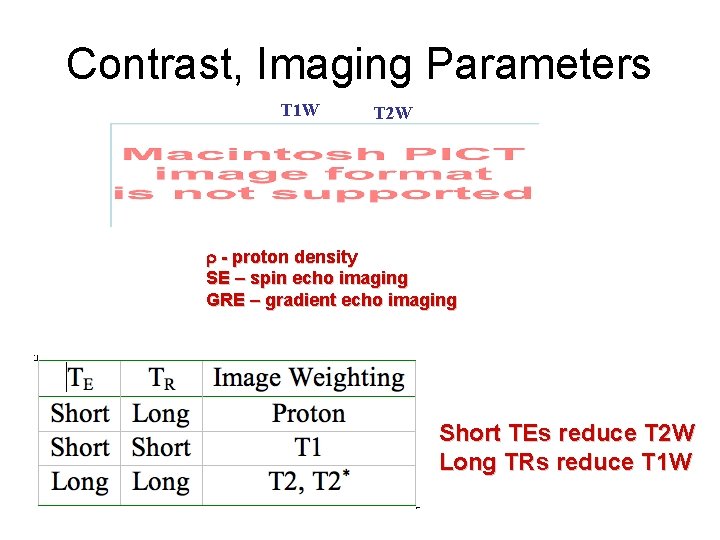
Contrast, Imaging Parameters T 1 W T 2 W r - proton density SE – spin echo imaging GRE – gradient echo imaging Short TEs reduce T 2 W Long TRs reduce T 1 W

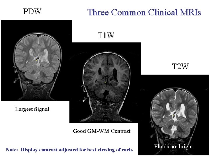
PDW Three Common Clinical MRIs T 1 W T 2 W Largest Signal Good GM-WM Contrast Note: Display contrast adjusted for best viewing of each. Fluids are bright

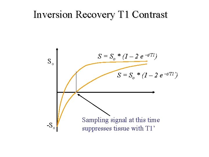
Inversion Recovery T 1 Contrast So S = So * (1 – 2 e –t/T 1) S = So * (1 – 2 e –t/T 1’) -So Sampling signal at this time suppresses tissue with T 1’

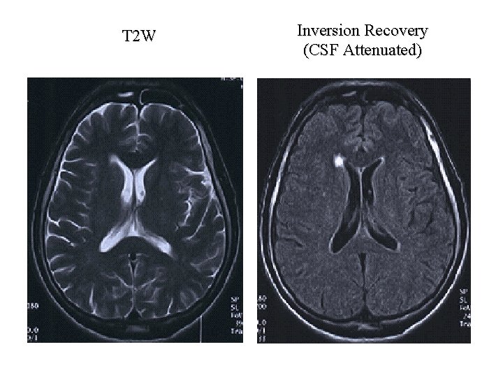
T 2 W Inversion Recovery (CSF Attenuated)

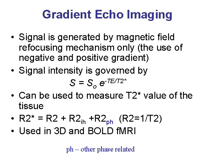
Gradient Echo Imaging • Signal is generated by magnetic field refocusing mechanism only (the use of negative and positive gradient) • Signal intensity is governed by S = So e-TE/T 2* • Can be used to measure T 2* value of the tissue • R 2* = R 2 + R 2 ih +R 2 ph (R 2=1/T 2) • Used in 3 D and BOLD f. MRI ph – other phase related

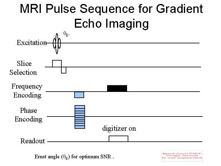
MRI Pulse Sequence for Gradient Echo Imaging E. Excitation Slice Selection Frequency Encoding Phase Encoding digitizer on Readout Ernst angle ( E) for optimum SNR.

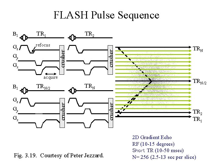
FLASH Pulse Sequence Gz refocus TR 2 crusher TR 1 crusher B 1 Gy Gx acquire Gy Gx Fig. 3. 19. Courtesy of Peter Jezzard. crusher Gz TRN/2 crusher B 1 TRN TR 2 TR 1 2 D Gradient Echo RF (10 -15 degrees) Short TR (10 -50 msec) N= 256 (2. 5 -13 sec per slice)

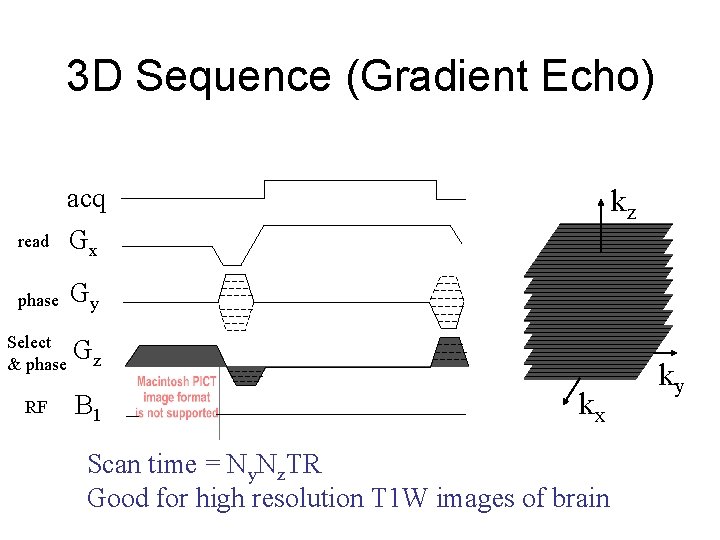
3 D Sequence (Gradient Echo) read acq Gx phase Gy Select & phase Gz RF B 1 kz kx Scan time = Ny. Nz. TR Good for high resolution T 1 W images of brain ky

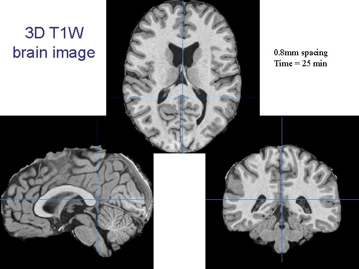
3 D T 1 W brain image 0. 8 mm spacing Time = 25 min

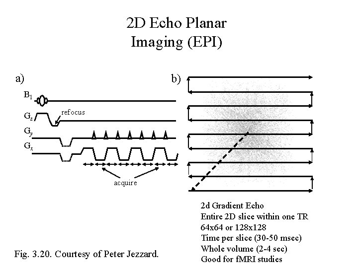
2 D Echo Planar Imaging (EPI) a) b) B 1 Gz refocus Gy Gx acquire Fig. 3. 20. Courtesy of Peter Jezzard. 2 d Gradient Echo Entire 2 D slice within one TR 64 x 64 or 128 x 128 Time per slice (30 -50 msec) Whole volume (2 -4 sec) Good for f. MRI studies

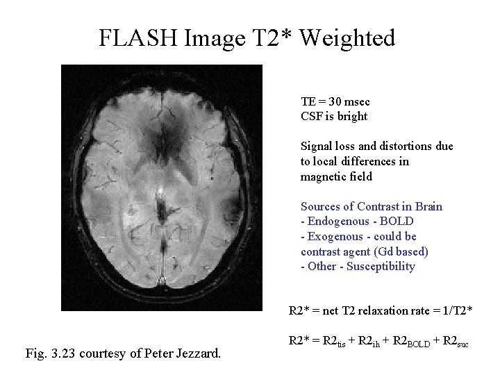
FLASH Image T 2* Weighted TE = 30 msec CSF is bright Signal loss and distortions due to local differences in magnetic field Sources of Contrast in Brain - Endogenous - BOLD - Exogenous - could be contrast agent (Gd based) - Other - Susceptibility R 2* = net T 2 relaxation rate = 1/T 2* Fig. 3. 23 courtesy of Peter Jezzard. R 2* = R 2 tis + R 2 ih + R 2 BOLD + R 2 suc

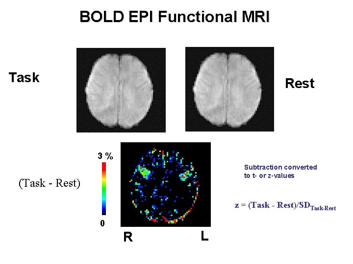
BOLD EPI Functional MRI Task Rest 3% Subtraction converted to t- or z-values (Task - Rest) z = (Task - Rest)/SDTask-Rest 0 R L

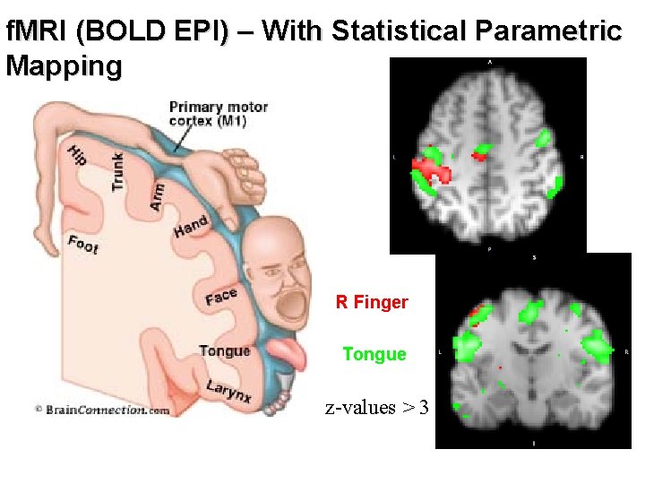
f. MRI (BOLD EPI) – With Statistical Parametric Mapping R Finger Tongue z-values > 3

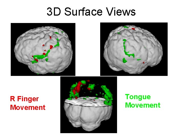
3 D Surface Views R Finger Movement Tongue Movement