Text Analytics Giuseppe Attardi Language Modeling IP notice

Text Analytics Giuseppe Attardi Language Modeling IP notice: some slides from: Dan Jurafsky, Jim Martin, Sandiway Fong, Dan Klein

Outline l Language Modeling (N-grams) N-gram Intro The Chain Rule The Shannon Visualization Method Evaluation: • Perplexity Smoothing: • Laplace (Add-1) • Add-prior

Probabilistic Language Model: Uses Goal: assign a probability to a sentence l Machine Translation: l P(high winds tonite) > P(large winds tonite) l Spell Correction “The o�ce is about fifteen minuets from my house" • P(about fifteen minutes from) l > P(about fifteen minuets from) Speech Recognition P(I saw a van) >> P(eyes awe of an) l Summarization, question answering, etc.

Why Language Models l We have an English speech recognition system, which answer is better? Speech Interpretation speech recognition system speech cognition system speck podcast histamine スピーチ が 救出 ストン l Language models tell us the answer!

Language Modeling l We want to compute P(w 1, w 2, w 3, w 4, w 5…wn) = P(W) = the probability of a sequence l Alternatively we want to compute P(w 5|w 1, w 2, w 3, w 4) = the probability of a word given some previous words l The model that computes P(W) or P(wn|w 1, w 2…wn-1) is called the language model. l A better term for this would be “The Grammar” l But “Language model” or LM is standard

Computing P(W) l How to compute this joint probability: P(“the”, “other”, “day”, “I”, “was”, “walking”, “along”, “and”, “saw”, “a”, “lizard”) l Intuition: let’s rely on the Chain Rule of Probability

The Chain Rule l Recall the definition of conditional probabilities l Rewriting: More generally P(A, B, C, D) = P(A)P(B|A)P(C|A, B)P(D|A, B, C) l In general l P(x 1, x 2, x 3, …xn) = P(x 1)P(x 2|x 1)P(x 3|x 1, x 2)…P(xn|x 1…xn-1)

The Chain Rule applied to joint probability of words in sentence P(“the big red dog was”) = P(the) • P(big|the) • P(red|the big) • P(dog|the big red) • P(was|the big red dog)

Obvious estimate l How to estimate? P(the | its water is so transparent that) = C(its water is so transparent that the) ________________________________________ C(its water is so transparent that)

Unfortunately l There a lot of possible sentences l We will never be able to get enough data to compute the statistics for those long prefixes P(lizard|the, other, day, I, was, walking, along, and, saw, a) or P(the|its water is so transparent that)

Markov Assumption l Make the simplifying assumption P(lizard|the, other, day, I, was, walking, along, and, saw, a) = P(lizard|a) l or maybe P(lizard|the, other, day, I, was, walking, along, and, saw, a) = P(lizard|saw, a)

Markov Assumption So for each component in the product, replace with the approximation (assuming a prefix of length N) Bigram model

N gram models We can extend to trigrams, 4 grams, 5 grams l In general this is an insu�cient model of language l because language has long distance dependencies: “The computers which I had just put into the machine room on the fifth floor crash often. ” l But we can often get away with N gram models

Estimating bigram probabilities l The Maximum Likelihood Estimate

An example <s> I am Sam </s> l <s> Sam I am </s> l <s> I do not like green eggs and ham </s> l l This is the Maximum Likelihood Estimate, because it is the one which maximizes P(Training set|Model)

Maximum Likelihood Estimates l The Maximum Likelihood Estimate of some parameter of a model M from a training set T is the estimate that maximizes the likelihood of the training set T given the model M Suppose the word “Chinese” occurs 400 times in a corpus of a million words (e. g. the Brown corpus) l What is the probability that a random word from some other text will be “Chinese” l MLE estimate is 400/1000000 =. 004 l This may be a bad estimate for some other corpus l But it is the estimate that makes it most likely that “Chinese” will occur 400 times in a million word corpus.

Maximum Likelihood We want to estimate the probability, p, that individuals are infected with a certain kind of parasite. The maximum likelihood Ind. Infected Probability of method (discrete distribution): observation 1 1 p 2 0 1–p 3 1 p 4 1 p 5 0 1–p 6 1 p 7 1 p 8 0 1–p 9 0 1–p 10 1 p 1. Write down the probability of each observation by using the model parameters 2. Write down the probability of all the data 3. Find the value parameter(s) that maximize this probability

Maximum likelihood We want to estimate the probability, p, that individuals are infected with a certain kind of parasite. Ind. Infected Probability of observation 1 1 p 2 0 1–p 3 1 p 4 1 p 5 0 1–p 6 1 p 7 1 p 8 0 1–p 9 0 1–p 10 1 p Likelihood function: - Find the value parameter(s) that maximize this probability

Computing the MLE l Set the derivative to 0: l Solutions: p=0 p=1 p = 0. 6 (minimum) (maximum)

More examples: Berkeley Restaurant Project l l l can you tell me about any good Cantonese restaurants close by mid priced thai food is what I’m looking for tell me about Chez Panisse can you give me a listing of the kinds of food that are available I’m looking for a good place to eat breakfast when is Caffe Venezia open during the day

Raw bigram counts l Out of 9222 sentences

Raw bigram probabilities l Normalize by unigrams (divide by C(w-1)): l Result:

Bigram estimates of sentence probabilities P(<s> I want english food </s>) = P(i|<s>) x P(want|I) x P(english|want) x P(food|english) x P(</s>|food) =. 000031

What kinds of knowledge? P(english|want) =. 0011 P(chinese|want) =. 0065 P(to|want) =. 66 P(eat | to) =. 28 P(food | to) = 0 P(want | spend) = 0 P(i | <s>) =. 25

Practical Issues l Compute in log space Avoid underflow Adding is faster than multiplying log(p 1 • p 2 • p 3 • p 4) = log(p 1) + log(p 2) + log(p 3) + log(p 4)

Shannon’s Game l What if we turn these models around and use them to generate random sentences that are like the sentences from which the model was derived. Jim Martin

The Shannon Visualization Method l l l Generate random sentences: Choose a random bigram <s>, w according to its probability Now choose a random bigram (w, x) according to its probability And so on until we choose </s> Then string the words together <s> I I want to to eat Chinese food </s>

Approximating Shakespeare l

Shakespeare as corpus l N=884, 647 tokens, V=29, 066 l Shakespeare produced 300, 000 bigram types out of V 2= 844 million possible bigrams: so, 99. 96% of the possible bigrams were never seen (have zero entries in the table) l Quadrigrams: What's coming out looks like Shakespeare because it is Shakespeare

The Wall Street Journal is not Shakespeare (no offense)

Lesson 1: the perils of overfitting l N-grams only work well for word prediction if the test corpus looks like the training corpus In real life, it often doesn’t We need to train robust models, adapt to test set, etc.

Train and Test Corpora l l A language model must be trained on a large corpus of text to estimate good parameter values. Model can be evaluated based on its ability to predict a high probability for a disjoint (held-out) test corpus (testing on the training corpus would give an optimistically biased estimate). Ideally, the training (and test) corpus should be representative of the actual application data. May need to adapt a general model to a small amount of new (in-domain) data by adding highly weighted small corpus to original training data.

Smoothing

Smoothing Since there a combinatorial number of possible word sequences, many rare (but not impossible) combinations never occur in training, so MLE incorrectly assigns zero to many parameters (aka sparse data). l If a new combination occurs during testing, it is given a probability of zero and the entire sequence gets a probability of zero (i. e. infinite perplexity). l In practice, parameters are smoothed (aka regularized) to reassign some probability mass to unseen events. l Adding probability mass to unseen events requires removing it from seen ones (discounting) in order to maintain a joint distribution that sums to 1.

Smoothing is like Robin Hood: Steal from the rich and give to the poor (in probability mass) Slide from Dan Klein

Laplace smoothing Also called add-one smoothing l Just add one to all the counts! l Very simple l MLE estimate: l l Laplace estimate: l Reconstructed counts:

Laplace smoothed bigram counts Berkeley Restaurant Corpus

Laplace smoothed bigrams

Reconstituted counts

Note big change to counts C(want to) went from 608 to 238! l P(to|want) from. 66 to. 26! l Discount d = c*/c l d for “chinese food” =. 10 A 10 x reduction! So in general, Laplace is a blunt instrument But Laplace smoothing not used for N-grams, as we have much better methods l Despite its flaws Laplace (add-k) is however still used to smooth other probabilistic models in NLP, especially l For pilot studies in domains where the number of zeros isn’t so huge.

Add k Add a small fraction instead of 1 l k = 0. 01 l

Even better: Bayesian unigram prior smoothing for bigrams l Maximum Likelihood Estimation l Laplace Smoothing l Bayesian Prior Smoothing

Lesson 2: zeros or not? l Zipf’s Law: l A small number of events occur with high frequency A large number of events occur with low frequency You can quickly collect statistics on the high frequency events You might have to wait an arbitrarily long time to get valid statistics on low frequency events Result: Our estimates are sparse! no counts at all for the vast bulk of things we want to estimate! Some of the zeroes in the table are really zeros But others are simply low frequency events you haven't seen yet. After all, ANYTHING CAN HAPPEN! How to address? l Answer: Estimate the likelihood of unseen N-grams! Slide from B. Dorr and J. Hirschberg

Zipf's law f 1/r (f proportional to 1/r) there is a constant k such that f r=k

Zipf's Law for the Brown Corpus

Zipf law: interpretation Principle of least effort: both the speaker and the hearer in communication try to minimize effort: Speakers tend to use a small vocabulary of common (shorter) words Hearers prefer a large vocabulary of rarer less ambiguous words Zipf's law is the result of this compromise Other laws … Number of meanings m of a word obeys the law: m 1/ f Inverse relationship between frequency and length

Practical Issues l We do everything in log space Avoid underflow (also adding is faster than multiplying)

Language Modeling Toolkits l SRILM http: //www. speech. sri. com/projects/srilm/ l IRSTLM l Ken LM

Google N Gram Release

Google Book N grams l http: //ngrams. googlelabs. com/

Google N Gram Release l l l l l serve serve serve as as as the the the incoming 92 incubator 99 independent 794 index 223 indication 72 indicator 120 indicators 45 indispensable 111 indispensible 40 individual 234 http: //googleresearch. blogspot. com/2006/08/all-our-n-gram-are-belong-to-you. html

Evaluation and Perplexity

Evaluation l l l l Train parameters of our model on a training set. How do we evaluate how well our model works? Look at the models performance on some new data This is what happens in the real world; we want to know how our model performs on data we haven’t seen Use a test set. A dataset which is different than our training set Then we need an evaluation metric to tell us how well our model is doing on the test set. One such metric is perplexity

Evaluating N gram models l Best evaluation for an N-gram Put model A in a task (language identification, speech recognizer, machine translation system) Run the task, get an accuracy for A (how many langs identified correctly, or Word Error Rate, or etc) Put model B in task, get accuracy for B Compare accuracy for A and B Extrinsic evaluation

Language Identification task Create an N gram model for each language l Compute the probability of a given text l Plang 1(text) Plang 2(text) Plang 3(text) l Select language with highest probability lang = argmaxl Pl(text)

Difficulty of extrinsic (in vivo) evaluation of N gram models l Extrinsic evaluation This is really time-consuming Can take days to run an experiment l So As a temporary solution, in order to run experiments To evaluate N-grams we often use an intrinsic evaluation, an approximation called perplexity But perplexity is a poor approximation unless the test data looks just like the training data So is generally only useful in pilot experiments (generally is not sufficient to publish)

Perplexity l The intuition behind perplexity as a measure is the notion of surprise. l How surprised is the language model when it sees the test set? Where surprise is a measure of. . . • Gee, I didn’t see that coming. . . The more surprised the model is, the lower the probability it assigned to the test set The higher the probability, the less surprised it was

Perplexity Measures of how well a model “fits” the test data. l Uses the probability that the model assigns to the test corpus. l Normalizes for the number of words in the test corpus and takes the inverse. l l Measures the weighted average branching factor in predicting the next word (lower is better).

Perplexity l Perplexity: l Chain rule: l For bigrams: l Minimizing perplexity is the same as maximizing probability The best language model is one that best predicts an unseen test set

Perplexity as branching factor How hard is the task of recognizing digits ‘ 0, 1, 2, 3, 4, 5, 6, 7, 8, 9’ l Perplexity: 10 l

Lower perplexity = better model l Model trained on 38 million words from the Wall Street Journal (WSJ) using a 19, 979 word vocabulary. l Evaluation on a disjoint set of 1. 5 million WSJ words. N-gram Order Perplexity Unigram 962 Bigram 170 Trigram 109

Unknown Words l How to handle words in the test corpus that did not occur in the training data, i. e. out of vocabulary (OOV) words? l Train a model that includes an explicit symbol for an unknown word (<UNK>): 1. Choose a vocabulary in advance and replace other words in the training corpus with <UNK>, or 2. Replace the first occurrence of each word in the training data with <UNK>.

Unknown Words handling l Training of <UNK> probabilities Create a fixed lexicon L of size V Any training word not in L changed to <UNK> Now we train its probabilities like a normal word l At decoding time In text input: use <UNK> probabilities for any word not in training

Smoothing

Advanced LM stuff l Current best smoothing algorithm Kneser-Ney smoothing l Other stuff Interpolation Backoff Variable-length n-grams Class-based n-grams Cache LMs Topic-based LMs Sentence mixture models Skipping LMs Parser-based LMs Word Embeddings • Clustering • Hand-built classes

Backoff and Interpolation l If we are estimating: Trigram P(z|xy) but C(xyz) is zero l Use info from: Bigram P(z|y) l Or even: Unigram P(z) l How to combine the trigram/bigram/unigram info?

Backoff versus interpolation l Backoff: use trigram if you have it, otherwise bigram, otherwise unigram l Interpolation: mix all three

Backoff Only use lower order model when data for higher order model is unavailable l Recursively back off to weaker models until data is available l Where P* is a discounted probability estimate to reserve mass for unseen events and ’s are back-off weights (see book for details).

Interpolation l Simple interpolation l Lambdas conditional on context:

How to set the lambdas? l Use a held-out corpus Training Data l Held Out Data Test Data Choose lambdas which maximize the probability of data i. e. fix the N-gram probabilities then search for lambda values that, when plugged into previous equation, give largest probability for held-out set Can use EM (Expectation Maximization) to do this search

Intuition of backoff+discounting l How much probability to assign to all the zero trigrams? Use Good-Turing or other discounting algorithm l How to divide that probability mass among different contexts? Use the N-1 gram estimates l What do we do for the unigram words not seen in training? Out Of Vocabulary = OOV words

Problem for N Grams: Long Distance Dependencies l Sometimes local context does not provide enough predictive clues, due to the presence of longdistance dependencies. Syntactic dependencies • “The man next to the large oak tree near the grocery store on the corner is tall. ” • “The men next to the large oak tree near the grocery store on the corner are tall. ” Semantic dependencies • “The bird next to the large oak tree near the grocery store on the corner flies rapidly. ” • “The man next to the large oak tree near the grocery store on the corner talks rapidly. ” l More complex models of language are needed to handle such dependencies.

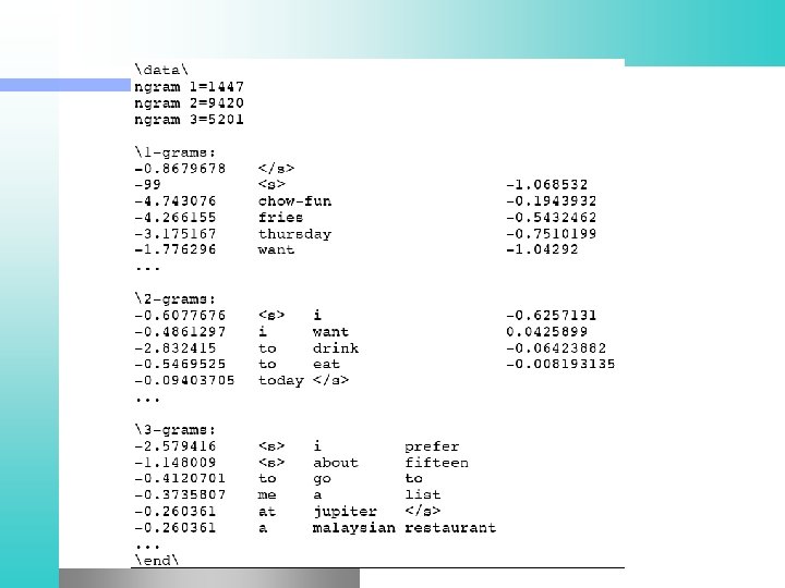
ARPA format

Language Models l l l Language models assign a probability that a sentence is a legal string in a language. They are useful as a component of many NLP systems, such as ASR, OCR, and MT. Simple N-gram models are easy to train on unsupervised corpora and can provide useful estimates of sentence likelihood. MLE gives inaccurate parameters for models trained on sparse data. Smoothing techniques adjust parameter estimates to account for unseen (but not impossible) events.

Exercise l Write two programs train unigram: Creates a unigram model test unigram: Reads a unigram model and calculates entropy and coverage for the test set l l Test them test/01 train input. txt test/01 test input. txt Train the model on data/wiki en train. word Calculate entropy and coverage on data/wiki entest. word Report your scores next week

Pseudo code: train unigram create a map counts create a variable total_count = 0 for each line in the training_file split line into an array of words append “</s>” to the end of words for each word in words add 1 to counts[word] add 1 to total_count open the model_file for writing for each word, count in counts probability = counts[word]/total_count print word, probability to model_file

Pseudo code: test unigram Load model create a map probabilities for each line in model_file split line into w and P set probabilities[w] = P Test and print for each line in test_file split line into an array of words append “</s>” to the end of words for each w in words add 1 to W set P = λunk / V if probabilities[w] exists set P += λ 1 * probabilities[w] else add 1 to unk add log 2 P to H print “entropy = ”+H/W print “coverage = ” + (W unk)/W

Summary l Language Modeling (N-grams) N-grams The Chain Rule The Shannon Visualization Method Evaluation: • Perplexity Smoothing: • Laplace (Add-1) • Add-k • Add-prior