Testing the home market effect in a multicountry

Testing the “home market effect” in a multi-country world: A theorybased approach Kristian Behrens, Andrea R. Lamorgese, Gianmarco I. P. Ottaviano, Takatoshi Tabuchi November 22, 2004

Purpose of the paper: To test and prove the presence of the “home market effect” in a multi-country world using extension of the two-country Krugman model to the multiple countries.

Two main explanations of the world trade phenomenon 1. Countries trade because they are somewhat different from one another: a country exports the goods that it is able to produce at relatively lower costs. Technology cross-country differences are reflected in Ricardian model, endowment differences – in Heckscher-Ohlin model. 2. Countries trade because of imperfect competition features - increasing returns to scale, product differentiation and market structure: a country exports the goods for which it offers a relatively large local demand, an outcome known as the “home market effect” (HME) – Krugman’s model.

Trade in different and similar goods (inter- and intra-industry trade) 1. Models based on cross-country differences (Ricardo and Heckscher-Ohlin) can only explain trade in different goods between different countries. Such trade is called inter-industry trade. 2. Trade in similar goods between similar countries is called intra-industry trade (for example, Germany both exports cars to Japan and imports cars from Japan, which is difficult to explain with models of comparative advantage). Similar goods are also referred to as varieties of the same good. Intraindustry trade can be rationalized with models featuring increasing returns to scale technology and love-of-variety preferences (Krugman).

Krugman’s model of international trade and home market effect Two-country economy with one factor of production (labor) and two sectors. One sector supplies a freely-traded homogeneous good under constant returns to scale and perfect competition, whereas the other sector produces a horizontally differentiated good under increasing returns and monopolistic competition. For each differentiated variety, fixed and marginal input requirements are constant and international trade is hampered by frictional trade costs of the “iceberg” type. Preferences are Cobb-Douglas across the two goods and symmetric CES between varieties of the differentiated good. Conclusion: Due to the fixed input requirement, the larger country supports in equilibrium the production of a more than proportionate number of differentiated varieties, thus being a net exporter of this good, displaying a HME.

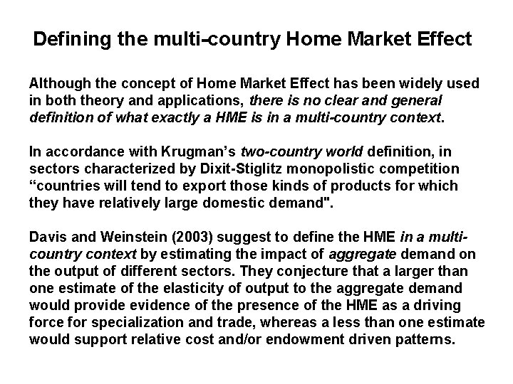
Defining the multi-country Home Market Effect Although the concept of Home Market Effect has been widely used in both theory and applications, there is no clear and general definition of what exactly a HME is in a multi-country context. In accordance with Krugman’s two-country world definition, in sectors characterized by Dixit-Stiglitz monopolistic competition “countries will tend to export those kinds of products for which they have relatively large domestic demand". Davis and Weinstein (2003) suggest to define the HME in a multicountry context by estimating the impact of aggregate demand on the output of different sectors. They conjecture that a larger than one estimate of the elasticity of output to the aggregate demand would provide evidence of the presence of the HME as a driving force for specialization and trade, whereas a less than one estimate would support relative cost and/or endowment driven patterns.

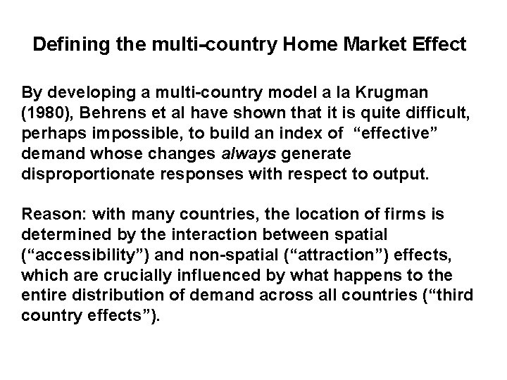
Defining the multi-country Home Market Effect By developing a multi-country model a la Krugman (1980), Behrens et al have shown that it is quite difficult, perhaps impossible, to build an index of “effective” demand whose changes always generate disproportionate responses with respect to output. Reason: with many countries, the location of firms is determined by the interaction between spatial (“accessibility”) and non-spatial (“attraction”) effects, which are crucially influenced by what happens to the entire distribution of demand across all countries (“third country effects”).

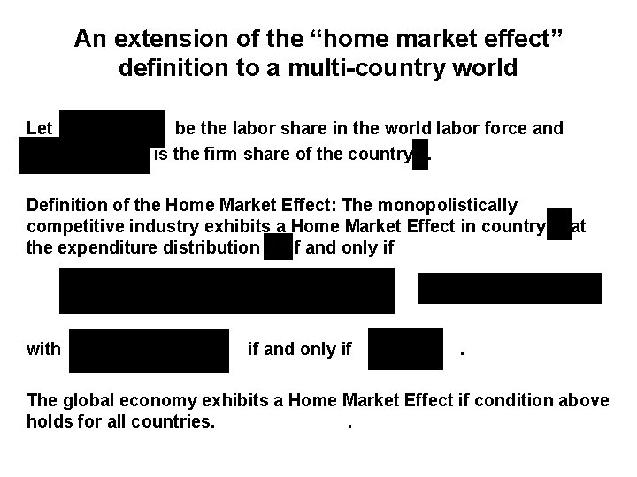
An extension of the “home market effect” definition to a multi-country world Let be the labor share in the world labor force and is the firm share of the country. Definition of the Home Market Effect: The monopolistically competitive industry exhibits a Home Market Effect in country the expenditure distribution if and only if with if and only if at . The global economy exhibits a Home Market Effect if condition above holds for all countries. .

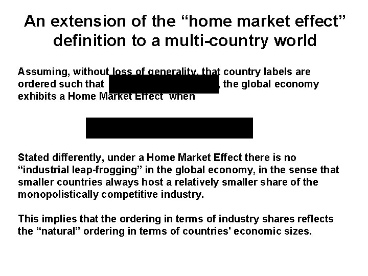
An extension of the “home market effect” definition to a multi-country world Assuming, without loss of generality, that country labels are ordered such that , the global economy exhibits a Home Market Effect when Stated differently, under a Home Market Effect there is no “industrial leap-frogging” in the global economy, in the sense that smaller countries always host a relatively smaller share of the monopolistically competitive industry. This implies that the ordering in terms of industry shares reflects the “natural” ordering in terms of countries' economic sizes.

Testing the multi-country Home Market Effect Conceptual difficulties do not imply the impossibility of assessing the role of product differentiation and market structure in shaping the structure of world trade. Behrens et al proposed a series of new theory-based non-parametric tests of the HME that are similar to the sign- and rank-tests used in the factor proportions literature. Main finding is that the empirical evidence strongly backs the HME prediction: local market size crucially matters in explaining and predicting observed trade flows, especially between OECD countries.

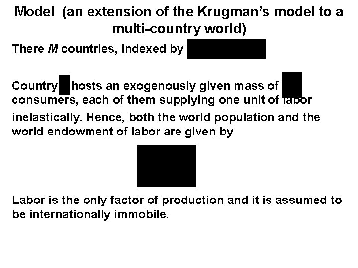
Model (an extension of the Krugman’s model to a multi-country world) There М countries, indexed by Country hosts an exogenously given mass of consumers, each of them supplying one unit of labor inelastically. Hence, both the world population and the world endowment of labor are given by Labor is the only factor of production and it is assumed to be internationally immobile.

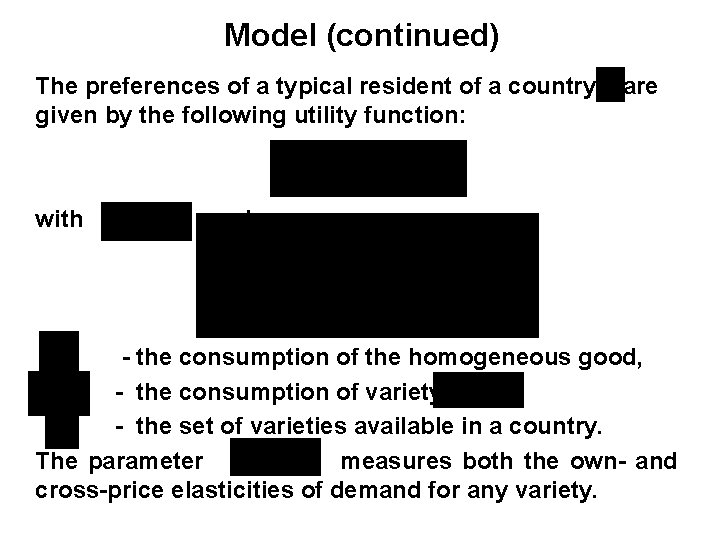
Model (continued) The preferences of a typical resident of a country given by the following utility function: with are and - the consumption of the homogeneous good, - the consumption of variety , - the set of varieties available in a country. The parameter measures both the own- and cross-price elasticities of demand for any variety.

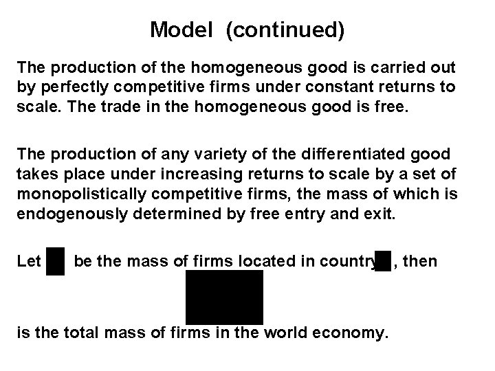
Model (continued) The production of the homogeneous good is carried out by perfectly competitive firms under constant returns to scale. The trade in the homogeneous good is free. The production of any variety of the differentiated good takes place under increasing returns to scale by a set of monopolistically competitive firms, the mass of which is endogenously determined by free entry and exit. Let be the mass of firms located in country , then is the total mass of firms in the world economy.

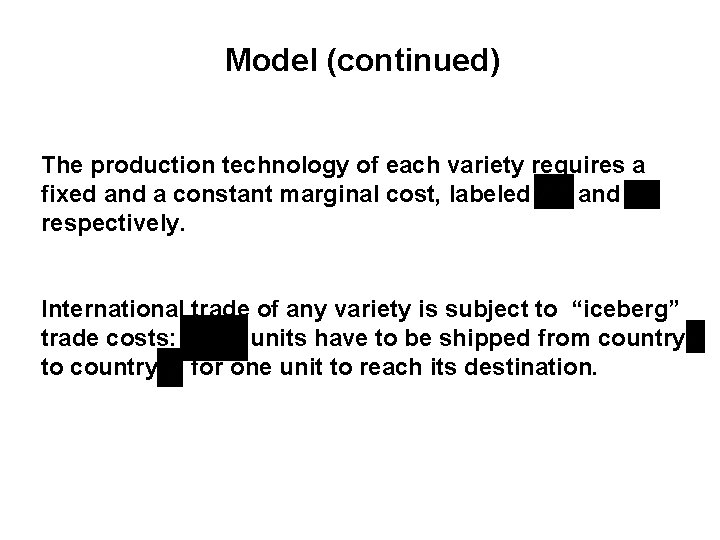
Model (continued) The production technology of each variety requires a fixed and a constant marginal cost, labeled and respectively. International trade of any variety is subject to “iceberg” trade costs: units have to be shipped from country to country for one unit to reach its destination.

Market equilibrium- homogeneous sector In the homogeneous sector perfect competition implies pricing at marginal cost, which, given the normalization of the unit input coefficient, is equal to the wage. As long as some homogeneous production takes place in all countries, free trade then generates factor price equalization (henceforth, FPE) across all countries. The homogeneous good is used as the numeraire, which implies that not only its price but also the wage equals one in all countries.

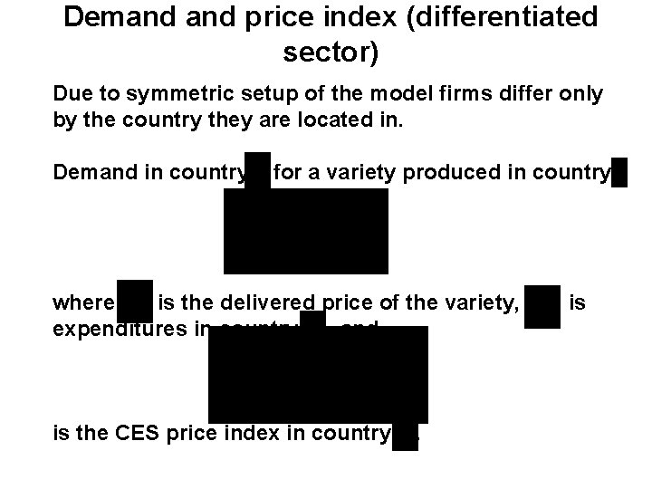
Demand price index (differentiated sector) Due to symmetric setup of the model firms differ only by the country they are located in. Demand in country for a variety produced in country where is the delivered price of the variety, expenditures in country , and is the CES price index in country . is

Firm’s optimization Because of the iceberg trade costs, a typical firm in country has to produce units to satisfy final demand in country. Any firm maximizes its own profit:

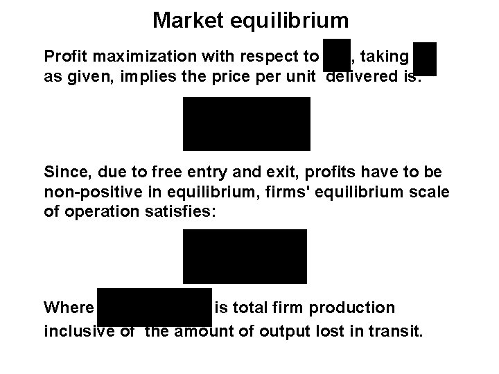
Market equilibrium Profit maximization with respect to , taking as given, implies the price per unit delivered is: Since, due to free entry and exit, profits have to be non-positive in equilibrium, firms' equilibrium scale of operation satisfies: Where is total firm production inclusive of the amount of output lost in transit.

Market equilibrium Using the market clearing condition, we can write the condition for non-positive profits for a typical variety produced in country as follows: which could be transformed into: where is a measure of trade freeness, valued one when trade is free ( ) and limiting zero when trade is inhibited ( ).

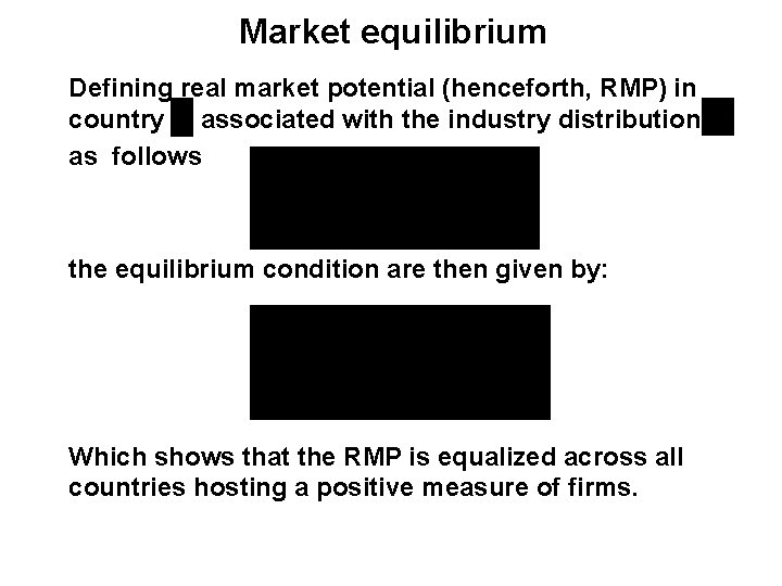
Market equilibrium If expression above holds as a strict inequality for country , then in equilibrium since no firm can break even there, whereas when expression above holds as an equality. Multiplying both sides of the expression above by the positive ‘s , and summing across countries, we get that in equilibrium the world mass of firms is constant and proportional to world population: This allows us to rewrite equilibrium condition in terms of shares:

Market equilibrium Defining real market potential (henceforth, RMP) in country associated with the industry distribution as follows the equilibrium condition are then given by: Which shows that the RMP is equalized across all countries hosting a positive measure of firms.

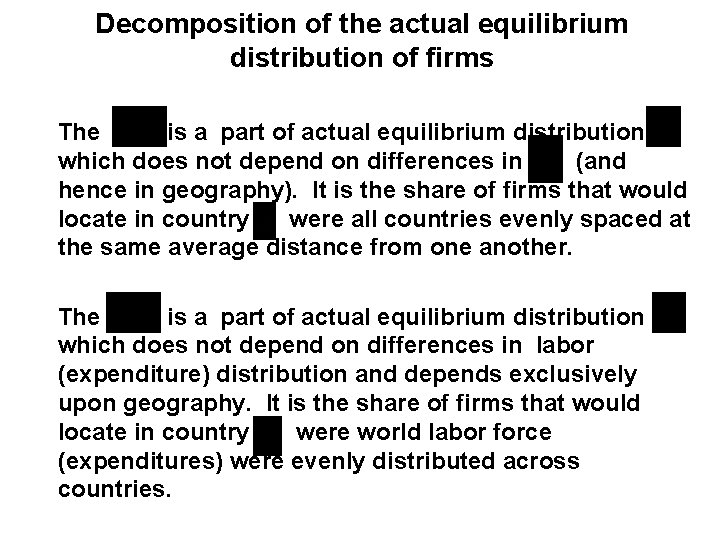
Decomposition of the actual equilibrium distribution of firms When the necessary condition for an interior equilibrium is satisfied, the equilibrium distribution of firms is given by and can be decomposed into two parts: where

Decomposition of the actual equilibrium distribution of firms The is a part of actual equilibrium distribution which does not depend on differences in (and hence in geography). It is the share of firms that would locate in country were all countries evenly spaced at the same average distance from one another. The is a part of actual equilibrium distribution which does not depend on differences in labor (expenditure) distribution and depends exclusively upon geography. It is the share of firms that would locate in country were world labor force (expenditures) were evenly distributed across countries.

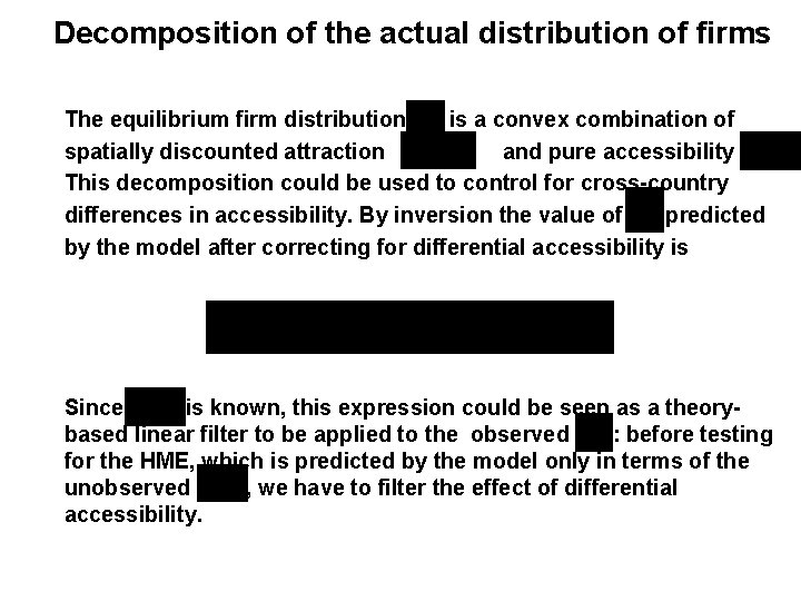
Decomposition of the actual distribution of firms The equilibrium firm distribution is a convex combination of spatially discounted attraction and pure accessibility. This decomposition could be used to control for cross-country differences in accessibility. By inversion the value of predicted by the model after correcting for differential accessibility is Since is known, this expression could be seen as a theorybased linear filter to be applied to the observed : before testing for the HME, which is predicted by the model only in terms of the unobserved , we have to filter the effect of differential accessibility.

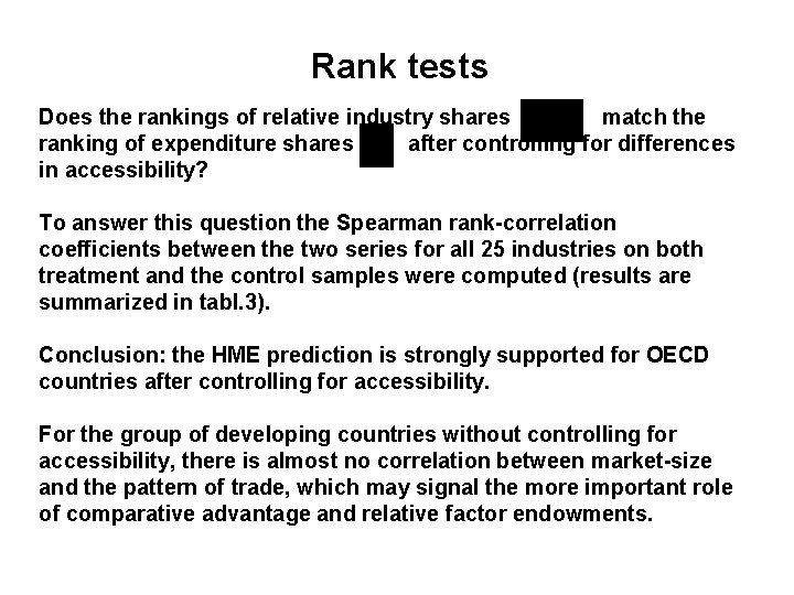
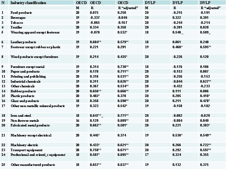
Rank tests Does the rankings of relative industry shares match the ranking of expenditure shares after controlling for differences in accessibility? To answer this question the Spearman rank-correlation coefficients between the two series for all 25 industries on both treatment and the control samples were computed (results are summarized in tabl. 3). Conclusion: the HME prediction is strongly supported for OECD countries after controlling for accessibility. For the group of developing countries without controlling for accessibility, there is almost no correlation between market-size and the pattern of trade, which may signal the more important role of comparative advantage and relative factor endowments.

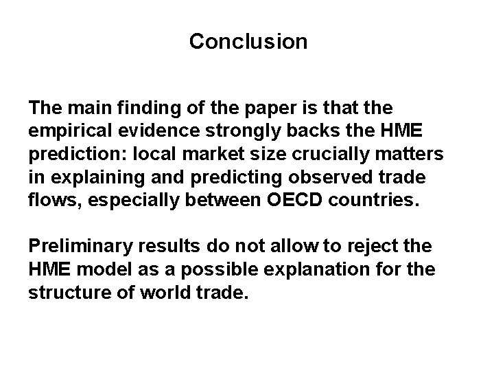
Conclusion The main finding of the paper is that the empirical evidence strongly backs the HME prediction: local market size crucially matters in explaining and predicting observed trade flows, especially between OECD countries. Preliminary results do not allow to reject the HME model as a possible explanation for the structure of world trade.

N Industry classification OECD DVLP 1 2 3 4 5 Food products Beverages Tobacco Textiles Wearing apparel except footwear M 20 19 19 20 19 R 0. 075 -0. 337 -0. 065 0. 334 -0. 070 R “adjusted” 0. 250 -0. 046 -0. 167 0. 358 0. 532* M 20 20 18 R -0. 215 0. 322 -0. 244 -0. 391 0. 548_ R “adjusted” -0. 191 0. 391 -0. 214 0. 020 0. 509_ 6 7 Leather products Footwear except rubber or plastic 19 19 0. 604** 0. 221 0. 579** 0. 291 18 19 0. 061 0. 460* 0. 240 0. 595** 8 Wood products except furniture 19 0. 214 0. 435* 20 -0. 226 0. 120 9 10 11 12 13 14 15 16 17 Furniture except metal Paper and products Printing and publishing Industrial chemicals Other chemicals Rubber products Plastic products Glass and products Other non-metallic mineral products 19 19 20 20 20 18 19 0. 314 0. 170 0. 316 0. 311 0. 367 0. 656** 0. 402* 0. 358 0. 323 0. 730** 0. 711** 0. 531** 0. 626** 0. 534** 0. 666** 0. 370 0. 598** 0. 542* 18 20 20 19 -0. 176 -0. 153 -0. 256 -0. 044 -0. 432 0. 111 0. 205 0. 211 -0. 158 0. 106 0. 087 -0. 153 0. 627** -0. 233 0. 086 0. 418* 0. 478* -0. 102 18 19 20 Iron and steel Non-ferrous metals Fabricated metal products 18 16 20 0. 647**_ 0. 129 0. 662** 0. 771** 0. 609** 0. 501* 20 18 20 -0. 002 -0. 084 0. 221 -0. 029 0. 049 0. 383* 21 Machinery except electrical 20 0. 445* 0. 374 19 0. 530* 0. 549** 22 23 24 Machinery electric Transport equipment Professional and scienti_c equipment 20 20 18 0. 433* 0. 758** 0. 507* 0. 621** 0. 671** 0. 695** 20 20 17 0. 266 0. 292 0. 324 0. 722** 0. 597** 0. 355 25 Other manufactured products 18 0. 657** 0. 637** 19 0. 132 0. 375