Test of Binary Mergers in Hierarchical Triples LR

Test of Binary Mergers in Hierarchical Triples LR w/ Zhong-Zhi Xianyu Induced Ellipticity for Inspiraling Binary Systems Lisa Randall (Harvard U. , Phys. Dept. ), Zhong-Zhi Xianyu (Harvard U. & Harvard U. , Dept. Math. ). Aug 28, 2017. 13 pp. Published in Astrophys. J. 853 (2018) no. 1, 93 e print: ar. Xiv: 1708. 08569 [gr-qc] | PDF An Analytical Portrait of Binary Mergers in Hierarchical Triple Systems Lisa Randall (Harvard U. ), Zhong-Zhi Xianyu (Harvard U. & Harvard U. ). Feb 15, 2018. e-Print: ar. Xiv: 1802. 05718 [gr-qc] | PDF A Direct Probe of Mass Density Near Inspiraling Binary Black Holes https: //arxiv. org/pdf/1805. 05335. pdf
 • Rates predicted")
Introduction • Successful GW detection of black hole mergers (and ns) • Rates predicted at tens/year • What can we learn? – – Black hole and neutron star physics! But what else? Environment? “New way to probe Universe” Should exist measurable, calculable differences due to tidal gravitational forces • Can tidal effects teach us about black hole neighborhoods? – Galaxy, globular cluster, isolated? – What observables should we consider and what can we hope to learn?

Inspiral “chirp Analytically Calculable As should be gravitational perturbations to it Merger History 3 stages: inspiral, merger, ringdown

Eccentricity • GWs circularize orbits – LIGO relies on circular templates • However, eccentricity can be generated from surrounding matter, and survive even if source only temporary – Potentially distinguish GN and SMBH, GC, isolated (natal kick) generation • Previously, studied numerically (eg Antonini, Perets) • Here present an analytical method for eccentricity distribution from galactic center black hole • Account for both tidal forces and evaporation caused by environment

Statistically Probe Merger Origins • Formation channels: – Isolated • Natal kick? – Dynamical: GC, SMBH • Hierarchical Triples • Observables: – Mass, spin, eccentricity • Integrate over initial distributions to find eccentricity distribution – Numerical, Analytical approaches • Insights from resulting distributions – True measure of utility depends on what numbers turn out to be

Review: GW Emission from Inspiraling Binary Assume circular, fixed orbit, point masses • Chirp mass: Mass quadrupole

Inspiral from GW: radius not fixed • Radiation power: • Energy: • Solve for

Generalize: Eccentric Orbit • Orbital frequency no longer constant Eccentric anomaly Polar coordinates

Sound and Shape of Eccentricity • No longer constant frequency • Higher harmonics • Quadrupole dominates for small e • Large e:

Eccentricity loss during infall • Use d. J/dt, d. E/dt from GW to derive • da/dt, de/dt =>a(e) Note base frequency ~1/a 3/2 a depends on e so even base frequency dependence reflects eccentricity

Measurable? • Large eccentricity: faster merger – Closer together – Higher harmonics • Small eccentricity – Can have small e, even if merger began with large e – Measurable with detailed measurement of waveform • Question become: can we drive eccentricity to larger values that survive into LIGO window? – Yes if we can drive e sufficiently – Assume e~o(. 01) can be measured – Source of post-formation eccentricity would be tidal forces

Rate: Tidal and GW modulation Perturbative :

Tidal generation of eccentricity • Competing effects – Gravitational wave emission throughout – Need coherent generation of eccentricity – Tidal force constant if nearby third body • Need a hierarchical triple – otherwise unstable • Can exist in cosmos – Galactic nuclei with SMBH – Dense globular clusters (binary-binary scattering)
 Point Source Tidal Force: Kozai Lidov • Perturb: • Ft/mv~")
Drive e with (eg) Point Source Tidal Force: Kozai Lidov • Perturb: • Ft/mv~ • Compare • Rate of change smaller than both inner and outer orbital frequencies; perturbative

Kozai-Lidov resonance : coherent generation Interchange between inclination and eccentricity |J|=const. |J 2|=const. J 2 J |J 1|∝(1 -e 2)1/2 J I I J 1 highly inclined J 1 highly eccentric

Critical Angle for Eccentricity to Develop Need High Inclination

Does eccentricity survive to LIGO? • Tidal modulation increases or decreases e • KL rate slower than orbital frequencies – Many orbits while e develops • But GW always decreases it • Need tidal effect to work fast enough that GW won’t erase it • Want tidal modulation frequency greater than circularization from GW rate

Tidal Sphere of Influence • Comparing rates of GW-circularization and tidal generation of eccentricity <1 >1 • Sufficiently large a : tidal modulation fast enough. Find critical separation—after GW dominates

So how much e remains? • Enters LIGO window Compare to binary orbit size when tidal force no longer dominates • Method I: Follow inspiral to LIGO a due to GW analytically • In first paper needed “initial” e distribution: note independent of background density profile so just one function • Then can find how much e lost as it inspirals

Second paper: analytical solution • Analytical solution at least in principle lets us relate measurable quantity (e) directly to parameters of environment in which BBH formed • Distribution of e depends on initial parameters • With solution, don’t need to numerically scan over all parameters • Can directly relate to density distribution • Key difference is included PN correction

Three-Body Systems Perturbative: hierarchical triples

Jacobi Coordinates: Hierarchical

Quadrupole Approx: Integrable System Angles to characterize both orbits Angles to characterize relative orbital planes Average over orbits (integrate out fast modes)

Exploit Hierarchy: Orbit-Orbit Coupling and Multipole Expansion

Averaged Hamiltonian Interaction

Aside: Delauney Variables Set of variables in which H 1, H 2 can be written entirely in terms of one variable • Tells us that in this set of variables a perturbation will induce slow change in orbit • This is what happens and how it is calculated

Analytical Computation of Final e • Need to include also PN correction • PN effect destroys resonance and allows GW to take over – No longer in tidal sphere of influence • • Want to know how much eccentricity remains First we calculate merger time Let’s consider examples to see how to do that Then we see how it helps for calculating eccentricity

Case I: fast merger

Opposite extreme: isolation limit
 Find lifetime of fictitious binary with the max")
We calculate: KL-boosted (but several cycles) Find lifetime of fictitious binary with the max e Correct for amount of time spent with that e

Merger Time Use sum of tidal and PN Hamiltonians Works well!!

What about eccentricity? • Now that we know merger time can postulate an isolated binary with that same merger time, mass, and same initial semi-major axis • Eccentricity distribution follows that of the isolated one in the end-- where KL turned off

KL: Interchange Conserved: Dynamical conjugate Use Delauney Then rewrite Argument of periapsis

Including precession of periapsis, GR Precession: incoherent with KL GR: back reaction GW (Peters Equation) as before: E, J no longer conserved Critical to calculation that change in orbital radius dominated by large eccentricity region

Summary Used to generate numerical solutions

Use changes occurring at largest e Take fictitious binary; same m 1, m 2, a 1, tmerger emax From PN and KL, tslow GW With equivalent e Use gw

Comparison to numerical results Works well away from large e

What to do with this result? Lots or parameters Only a few relevant Make some assumptions: hopefully test in the end thermal Distribution in a 2 tells us about density distribution of black holes--origin Core vs cusp:

Additional constraints: Evaporation and Tidal Disruption This was all for an isolated binary in presence of BH In reality, binary inside galaxy Evaporation can occur: depends on L To date, competition done with simulation In first analysis we used a cutoff L beyond which evaporation dominates • Now with analytical result, we can compare to analytical result for evaporation • • • We also require no tidal disruption from SMBH

Evaporation and disruption • Evaporation of binaries by scattering with ambient matter: require merge, not evaporate Tidal disruption constraint:
 for solar mass")
Sample Result with all Constraints Cusp model: e>. 01: 5% (25%) for solar mass (10 solar mass) objects Should occur at measurable rate

Can in principle use to distinguish different density distributions • Eg Core vs Cusp, Different masses Background and bh distributions: bh number density, background matter density Cusp: α=7/4, β=2; Core: α=. 5, β=. 5 α=7/4, β=2, α=7/4, β=7/4 ,

Also some analytical understanding of dependencies Big initial e, small final e Very large I Vs smaller I and suppressed PN Interesting that m, a dependence reversed In end, first case dominates: stronger dependence and more of parameter space

Early stages but promising • Analytical result means we don’t have to calculate e distribution numerically • Only numerics is integrating over initial parameters – No Monte Carlo • Will however require lots of statistics in end • Also sometimes near SMBH, sometimes isolated (natal kicks), sometimes GN • We want to find ways to distinguish options • Or disentangle components • Clearly LISA can help • First observe ---then follow • Constraint on when e generated

At least as interesting… • LISA observes events for a few years • For certain parameter ranges, can monitor time evolution • Study change in orbital parameters • Direct probe of ambient density distribution

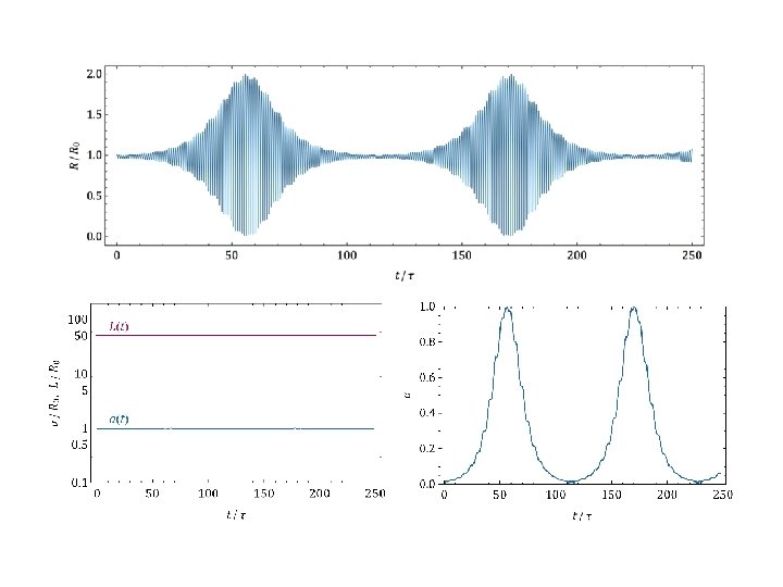
Longitudinal Doppler Shift • For now, consider orbit along line of slight • Velocity variation sum of min max velocities • Use energy conservation

Doppler Shift • Need visible shift f Δv • Need period < time in LISA window – Large f to improve resolution? Small a 1

Sample results

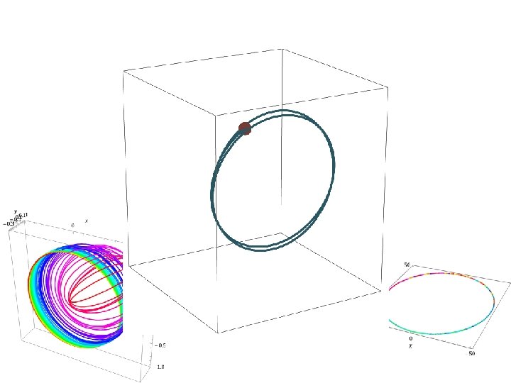
Real-time Eccentricity Generation • Can do similar analysis with e Favors large a 1

Results

Conclusions • Clearly information is there – Want to know where black holes come from – Distributions of matter surrounding them – Ultimately is it standard or nonstandard • Goal to retrieve the information • Early stages so hopeful!
 of finding a binary BH by LIGO with eccentricity e in")
The probability p(e) of finding a binary BH by LIGO with eccentricity e in a galactic nuclei, computed with assuming e 2 distribution at the sphere-of-influenceexit and with outer cutoff from evaporation.
 assuming n=0 as a function of the")
m=M☉ m=10 M☉ The probability p(e>0. 1) assuming n=0 as a function of the distance between the binary system and the center of a SMBH of mass 106 M☉
=e 2, e, 1 } emin=0. 5 The probability")
Effects of varying the e-distribution. ft(e)=e 2, e, 1 } emin=0. 5 The probability p(e>emin) of observing a binary BH in galactic nuclei with eccentricity larger than a given value emin by LIGO, as a function of cutoff distance Lcut. Distribution probably weighed to larger n since easier merger—bigger probability

Mass segregated: r-2 Core The probability of observing a binary BH in galactic nuclei with eccentricity e located at a distance L from the central BH. Evap, KL both most effective in central region. Outer region bigger volume but distribution falling.

Conclusions • Insights into understanding magnitude of eccentricity • Ultimate goal to scan through matter and BH profiles • Eccentricity distribution can be determined in relatively simple way • More work to get analytic understanding of e distribution before GW and also cutoff • Ultimately want to determine fast, slow mergers • GNs, globular clusters • High low eccentricities • One of most exciting programs on horizon • Very promising!
- Slides: 58