Term Structure Models Victor Lapshin Ph D research

Term Structure Models Victor Lapshin, Ph. D, research fellow at Higher School of Economics, Moscow, Russia

What is “Yield”? • Term structure of interest rates. • [Zero-Coupon] [Spot] Yield Curve. • Discount function. • We apply the terms “Yield” and “Interest Rate” interchangeably to either a loan interest rate or a deposit yield.

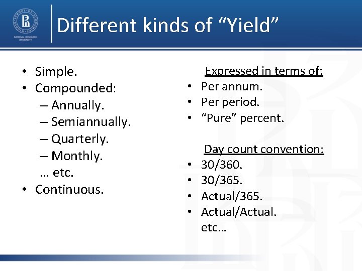
Different kinds of “Yield” • Simple. • Compounded: – Annually. – Semiannually. – Quarterly. – Monthly. … etc. • Continuous. Expressed in terms of: • Per annum. • Per period. • “Pure” percent. • • Day count convention: 30/360. 30/365. Actual/Actual. etc…

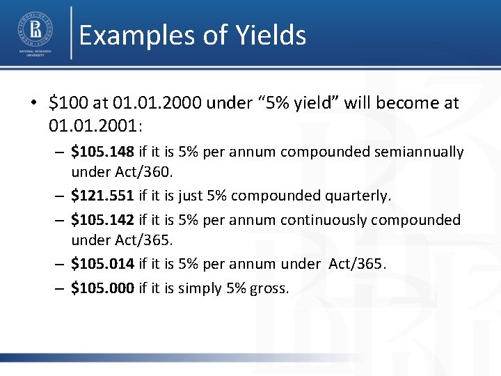
Examples of Yields • $100 at 01. 2000 under “ 5% yield” will become at 01. 2001: – $105. 148 if it is 5% per annum compounded semiannually under Act/360. – $121. 551 if it is just 5% compounded quarterly. – $105. 142 if it is 5% per annum continuously compounded under Act/365. – $105. 014 if it is 5% per annum under Act/365. – $105. 000 if it is simply 5% gross.

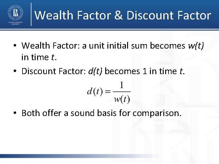
Wealth Factor & Discount Factor • Wealth Factor: a unit initial sum becomes w(t) in time t. • Discount Factor: d(t) becomes 1 in time t. • Both offer a sound basis for comparison.

Subjectivity of d and w • Wealth and discount factors depend on: – Whether we lend or borrow money. – Contract details. – Counterparty’s and our own credit risk. – Embedded options. …etc. • We need a way to objectively price instruments promising future cash flows.

Present Value • Given a description of a financial instrument determine its “present value”. • The problem admits different solutions. • We need some basic assumptions.

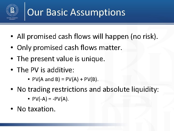
Our Basic Assumptions • • All promised cash flows will happen (no risk). Only promised cash flows matter. The present value is unique. The PV is additive: • PV(A and B) = PV(A) + PV(B). • No trading restrictions and absolute liquidity: • PV(-A) = -PV(A). • No taxation.

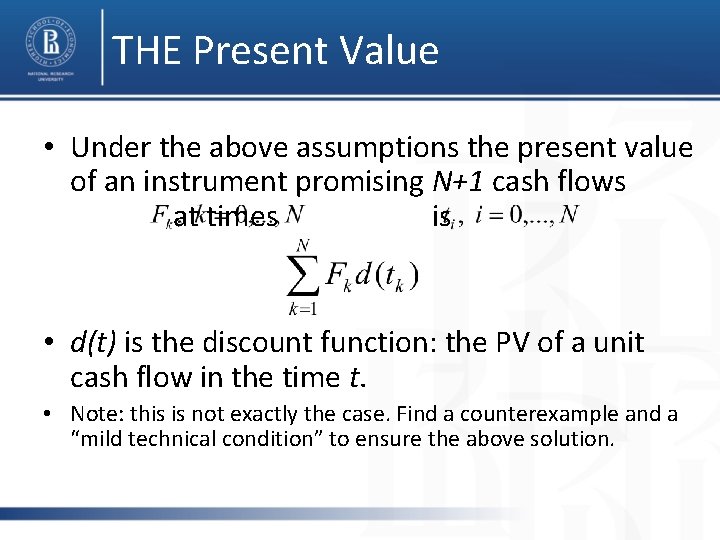
THE Present Value • Under the above assumptions the present value of an instrument promising N+1 cash flows at times is • d(t) is the discount function: the PV of a unit cash flow in the time t. • Note: this is not exactly the case. Find a counterexample and a “mild technical condition” to ensure the above solution.

The Discount Function • Suppose that Present Value = Opportunity Cost. • There is an “ideal market” where one can invest any amount (possibly, negative) of money for any term (equiv. bonds of all maturities and face values are traded). • Then d(t) is the current price of a bond with time t to maturity and unit face value.

The Problem • Find the discount function. • Available data: – Bond prices. – Bond descriptions. • Easy? • Do we really observe PV? • How do the observed values correspond to the PV? • What really are the observed values?

Formalizations • What is a “bond price”? – Closing price. • What if it wasn’t traded? • What if we desire an intraday estimation? – Last trade price. • What if no trades? • What if trades are unreliable (very small volume)? • Timing issues. – Bid & Ask quotes • Is “Price” a single number? • What if only one quote is present? • What if they are unreliable?

Dynamic & Static Models • Timing issues: – Bond A was priced at 12: 00. – Bond B was priced at 13: 00. – Were they both priced with respect to the same “true” discount function? • Does the discount function change over time? How? More assumptions. • We assume the static model.

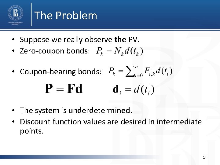
The Problem • Suppose we really observe the PV. • Zero-coupon bonds: • Coupon-bearing bonds: • The system is underdetermined. • Discount function values are desired in intermediate points. 14

More Assumptions • We have too little data available => we need more a priori assumptions. • Different assumptions lead to different problem formulations and to different results. – On the exact parametric form of the discount function (parametric methods). – On some extreme properties of the discount function (spline methods).

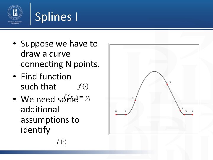
Splines I • Suppose we have to draw a curve connecting N points. • Find function such that • We need some additional assumptions to identify

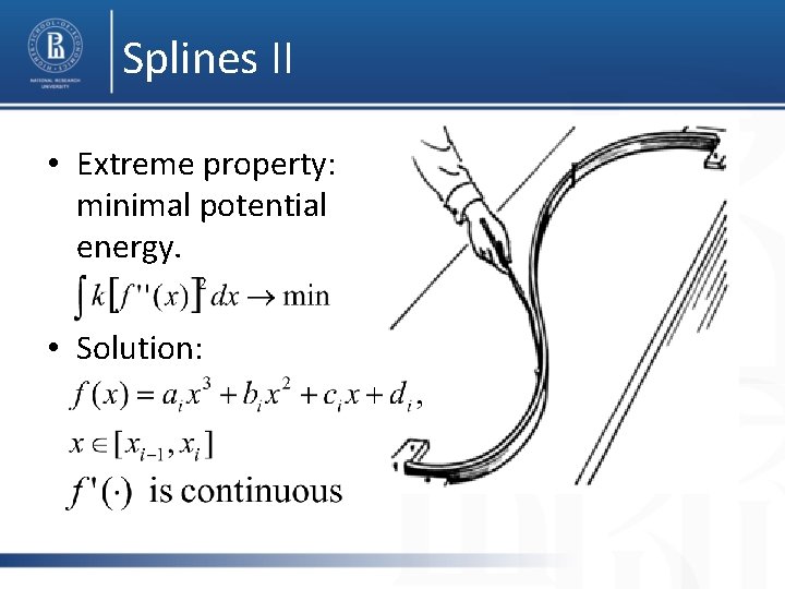
Splines II • Extreme property: minimal potential energy. • Solution:

Word Usage • If we postulate spline nature of the discount function, it is a parametric method (we assume a specific functional form).

Yield Curve • Assume continuous compounding: • t is the time: [t] = year. • r(t) is the continuously compounded yearly interest rate: [r(t)] = 1 / year.

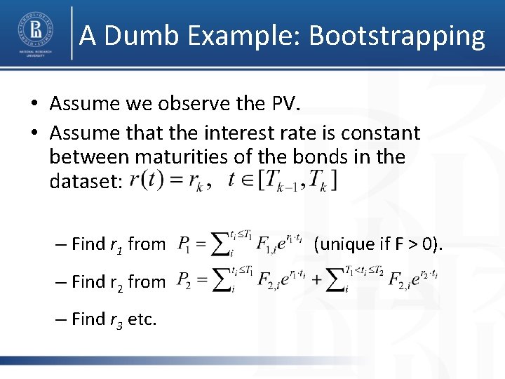
A Dumb Example: Bootstrapping • Assume we observe the PV. • Assume that the interest rate is constant between maturities of the bonds in the dataset: – Find r 1 from – Find r 2 from – Find r 3 etc. (unique if F > 0).

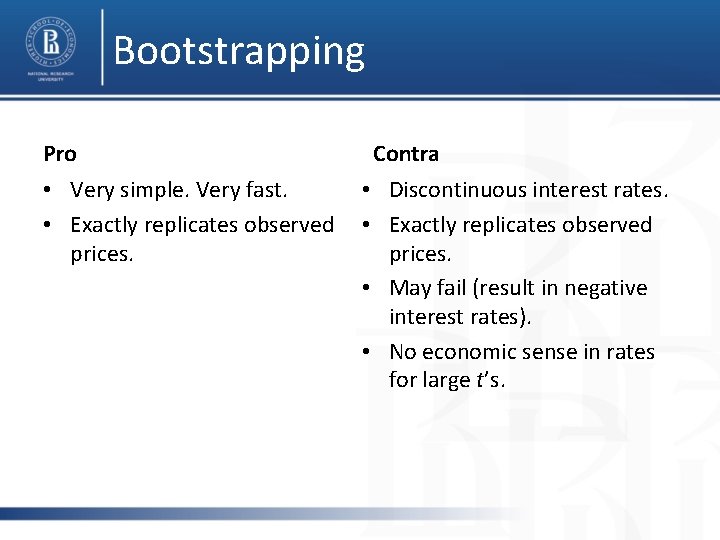
Bootstrapping Pro • Very simple. Very fast. • Exactly replicates observed prices. Contra • Discontinuous interest rates. • Exactly replicates observed prices. • May fail (result in negative interest rates). • No economic sense in rates for large t’s.

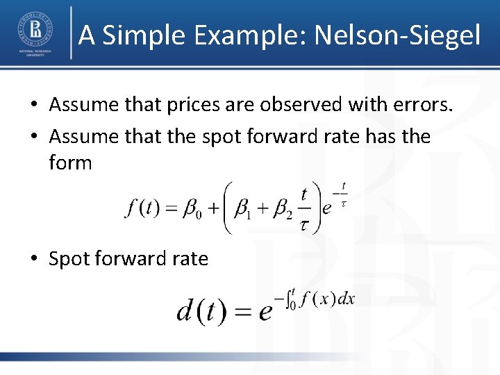
A Simple Example: Nelson-Siegel • Assume that prices are observed with errors. • Assume that the spot forward rate has the form • Spot forward rate

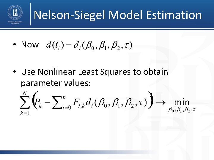
Nelson-Siegel Model Estimation • Now • Use Nonlinear Least Squares to obtain parameter values:

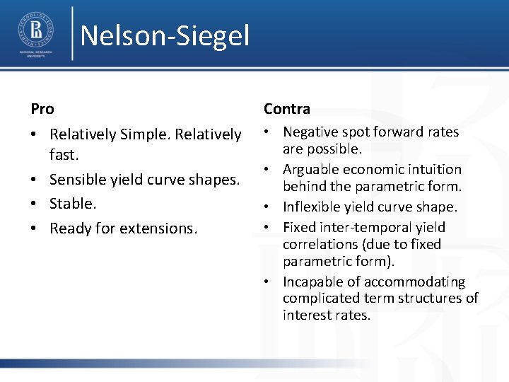
Nelson-Siegel Pro Contra • Relatively Simple. Relatively fast. • Sensible yield curve shapes. • Stable. • Ready for extensions. • Negative spot forward rates are possible. • Arguable economic intuition behind the parametric form. • Inflexible yield curve shape. • Fixed inter-temporal yield correlations (due to fixed parametric form). • Incapable of accommodating complicated term structures of interest rates.

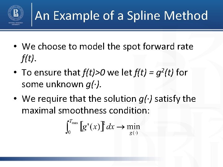
An Example of a Spline Method • We choose to model the spot forward rate f(t). • To ensure that f(t)>0 we let f(t) = g 2(t) for some unknown g(∙). • We require that the solution g(∙) satisfy the maximal smoothness condition:

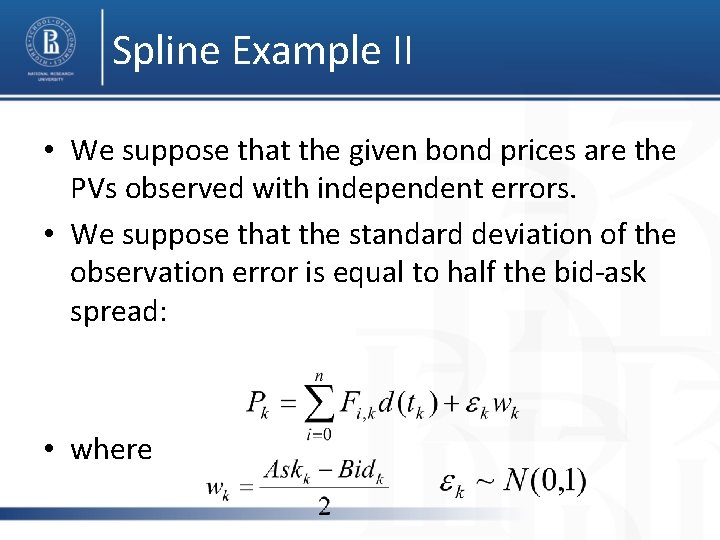
Spline Example II • We suppose that the given bond prices are the PVs observed with independent errors. • We suppose that the standard deviation of the observation error is equal to half the bid-ask spread: • where

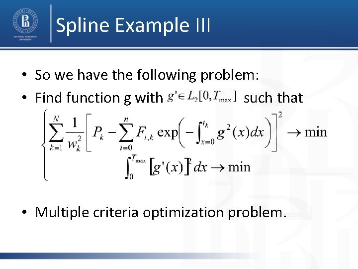
Spline Example III • So we have the following problem: • Find function g with such that • Multiple criteria optimization problem.

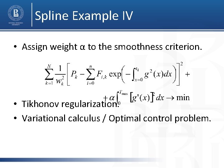
Spline Example IV • Assign weight α to the smoothness criterion. • Tikhonov regularization. • Variational calculus / Optimal control problem.

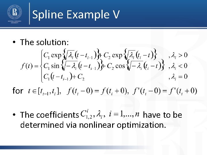
Spline Example V • The solution: for • The coefficients have to be determined via nonlinear optimization.

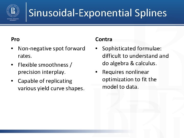
Sinusoidal-Exponential Splines Pro Contra • Non-negative spot forward rates. • Flexible smoothness / precision interplay. • Capable of replicating various yield curve shapes. • Sophisticated formulae: difficult to understand do algebra & calculus. • Requires nonlinear optimization to fit the model to data.

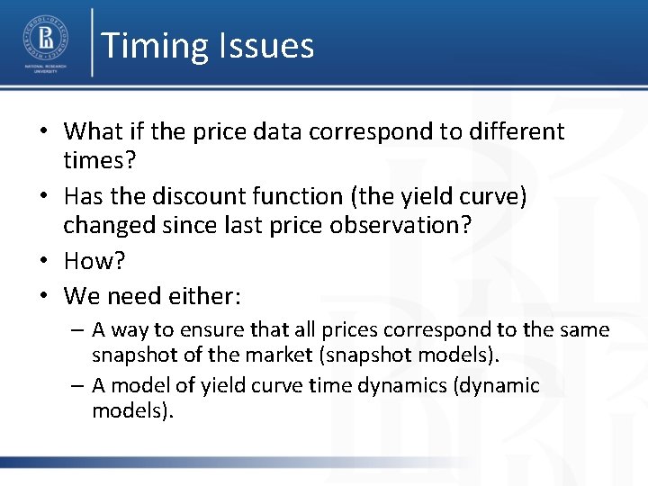
Timing Issues • What if the price data correspond to different times? • Has the discount function (the yield curve) changed since last price observation? • How? • We need either: – A way to ensure that all prices correspond to the same snapshot of the market (snapshot models). – A model of yield curve time dynamics (dynamic models).

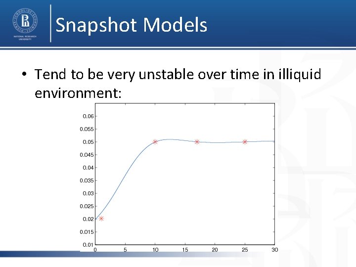
Snapshot Models • Tend to be very unstable over time in illiquid environment:

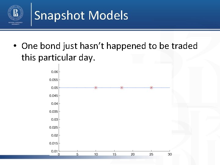
Snapshot Models • One bond just hasn’t happened to be traded this particular day.

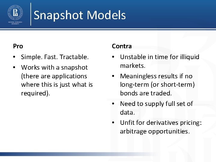
Snapshot Models Pro Contra • Simple. Fast. Tractable. • Works with a snapshot (there applications where this is just what is required). • Unstable in time for illiquid markets. • Meaningless results if no long-term (or short-term) bonds are traded. • Need to supply full set of data. • Unfit for derivatives pricing: arbitrage opportunities.

Dynamic Models • We need a way to describe the stochastic dynamics of the entire yield curve. – Simplify the problem. – Employ “higher maths”.

Simplified Dynamic Models • Model only finite number of key parameters: – Instantaneous (spot) interest rate. – Spot and long rates. – Yields for several key terms. – Several general factors. …etc. • The yield curve (all forward rates) may be derived from the stochastic dynamics of parameters (even if it’s a single spot rate). – Forward rate = “expected” future rate (have to consider risk-neutrality issues).

Simple Models Dynamic -> static Static -> dynamic • Low-dimensional dynamic models imply non-realistic zero-coupon yield curves: negative or infinite. • Consistency problems: arbitrage opportunities.

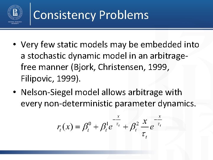
Consistency Problems • Very few static models may be embedded into a stochastic dynamic model in an arbitragefree manner (Bjork, Christensen, 1999, Filipovic, 1999). • Nelson-Siegel model allows arbitrage with every non-deterministic parameter dynamics.

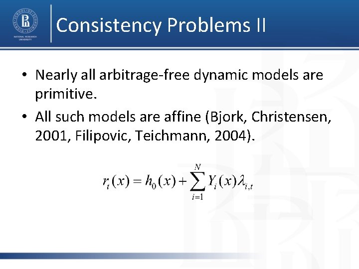
Consistency Problems II • Nearly all arbitrage-free dynamic models are primitive. • All such models are affine (Bjork, Christensen, 2001, Filipovic, Teichmann, 2004).

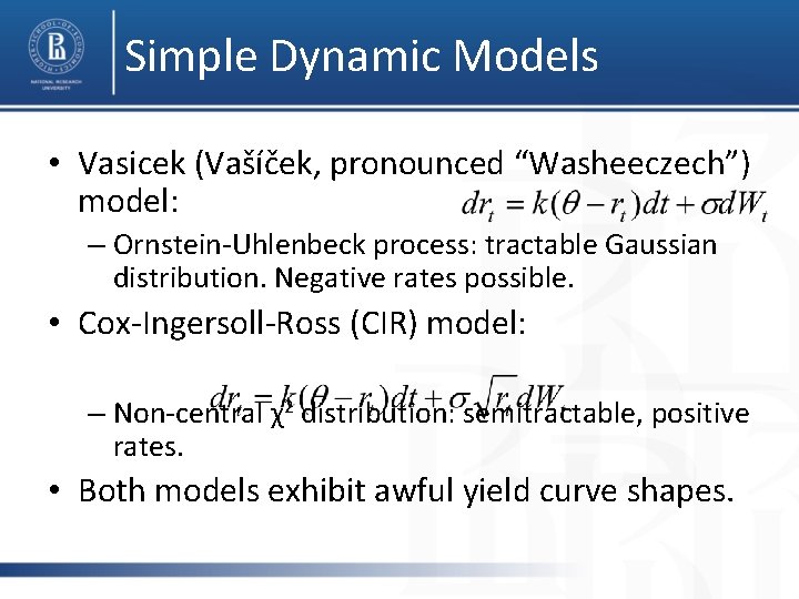
Simple Dynamic Models • Vasicek (Vašíček, pronounced “Washeeczech”) model: – Ornstein-Uhlenbeck process: tractable Gaussian distribution. Negative rates possible. • Cox-Ingersoll-Ross (CIR) model: – Non-central χ2 distribution: semitractable, positive rates. • Both models exhibit awful yield curve shapes.

Simple Dynamic Models Pro • • Simple. Dynamic. Sometimes tractable. Simple simulation. Relatively simple parameter inference. Contra • Incompatible with snapshot models (unrealistic yield curve shapes). • Unrealistic. • Inflexible.

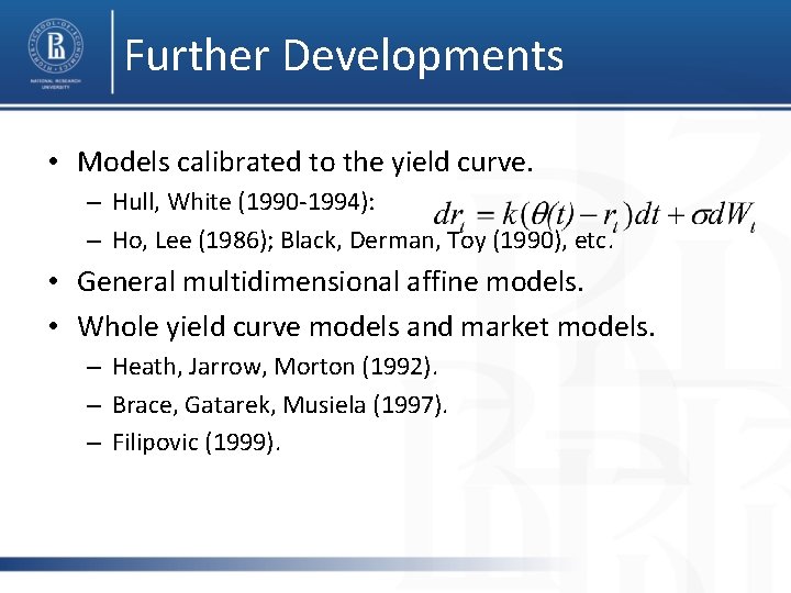
Further Developments • Models calibrated to the yield curve. – Hull, White (1990 -1994): – Ho, Lee (1986); Black, Derman, Toy (1990), etc. • General multidimensional affine models. • Whole yield curve models and market models. – Heath, Jarrow, Morton (1992). – Brace, Gatarek, Musiela (1997). – Filipovic (1999).

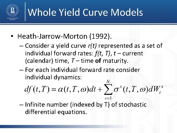
Whole Yield Curve Models • Heath-Jarrow-Morton (1992). – Consider a yield curve r(t) represented as a set of individual forward rates: f(t, T), t – current (calendar) time, T – time of maturity. – For each individual forward rate consider individual dynamics: – Infinite number (indexed by T) of stochastic differential equations.

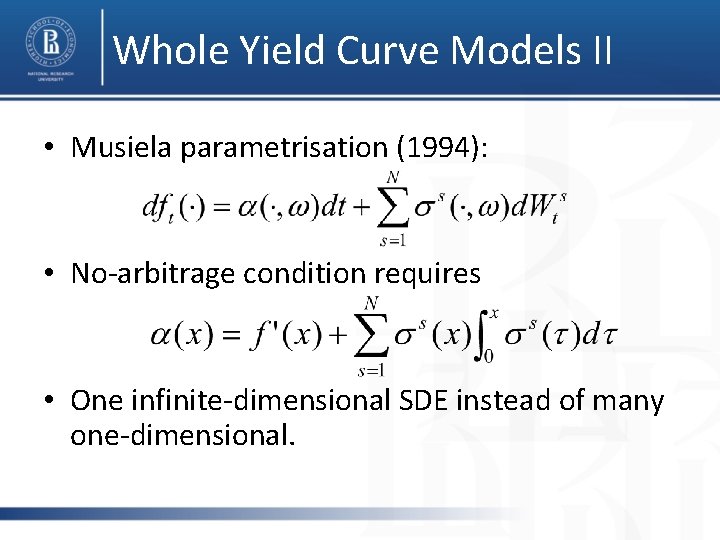
Whole Yield Curve Models II • Musiela parametrisation (1994): • No-arbitrage condition requires • One infinite-dimensional SDE instead of many one-dimensional.

vlapshin@hse. ru