Tensors and Component Analysis Musawir Ali Tensor Generalization

Tensors and Component Analysis Musawir Ali

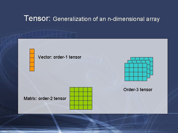
Tensor: Generalization of an n-dimensional array Vector: order-1 tensor Order-3 tensor Matrix: order-2 tensor

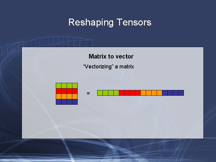
Reshaping Tensors Matrix to vector “Vectorizing” a matrix =

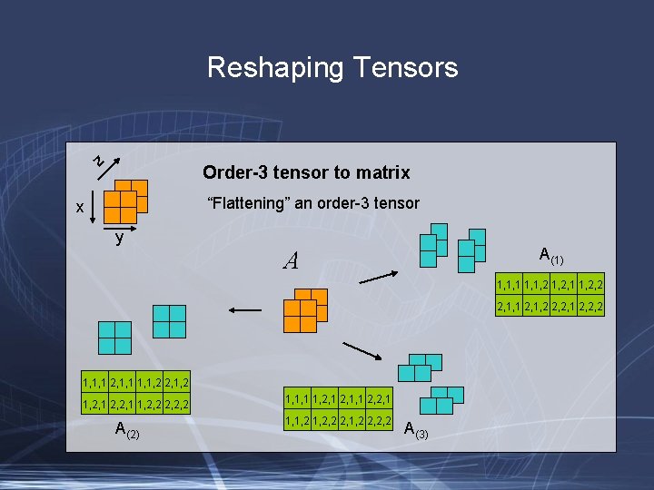
Reshaping Tensors z Order-3 tensor to matrix “Flattening” an order-3 tensor x y A(1) A 1, 1, 1, 2, 1 1, 2, 2 2, 1, 1 2, 1, 2 2, 2, 1 2, 2, 2 1, 1, 1 2, 1, 1, 2 2, 1, 2, 1 2, 2, 1 1, 2, 2, 2 A(2) 1, 1, 1 1, 2, 1, 1 2, 2, 1 1, 1, 2, 2 2, 1, 2 2, 2, 2 A(3)

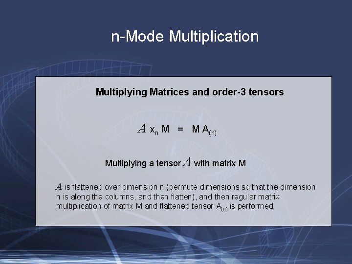
n-Mode Multiplication Multiplying Matrices and order-3 tensors A xn M = M A(n) Multiplying a tensor A with matrix M A is flattened over dimension n (permute dimensions so that the dimension n is along the columns, and then flatten), and then regular matrix multiplication of matrix M and flattened tensor A(n) is performed

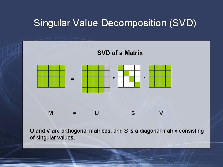
Singular Value Decomposition (SVD) SVD of a Matrix = M = * U * S VT U and V are orthogonal matrices, and S is a diagonal matrix consisting of singular values.

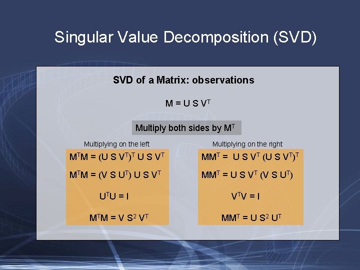
Singular Value Decomposition (SVD) SVD of a Matrix: observations M = U S VT Multiply both sides by MT Multiplying on the left Multiplying on the right MTM = (U S VT)T U S VT MMT = U S VT (U S VT)T MTM = (V S UT) U S VT MMT = U S VT (V S UT) U TU = I V TV = I M TM = V S 2 V T MMT = U S 2 UT

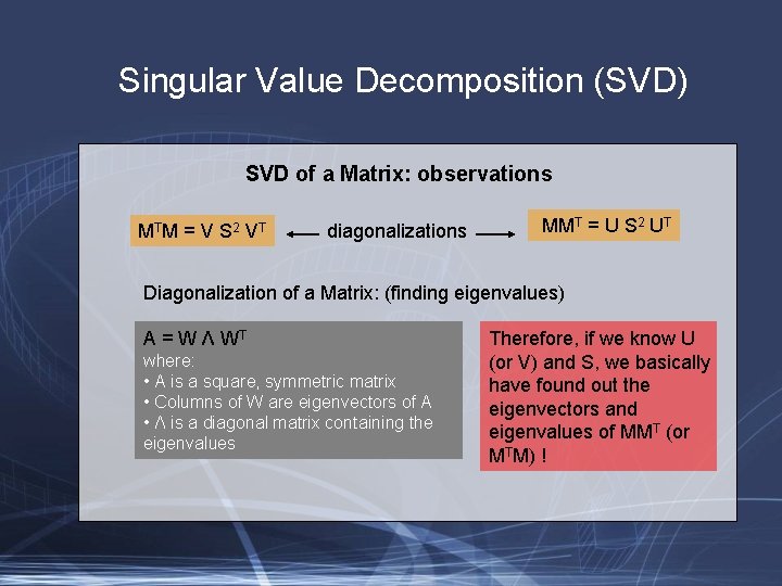
Singular Value Decomposition (SVD) SVD of a Matrix: observations MT M = V S 2 V T diagonalizations MMT = U S 2 UT Diagonalization of a Matrix: (finding eigenvalues) A = W Λ WT where: • A is a square, symmetric matrix • Columns of W are eigenvectors of A • Λ is a diagonal matrix containing the eigenvalues Therefore, if we know U (or V) and S, we basically have found out the eigenvectors and eigenvalues of MMT (or MTM) !

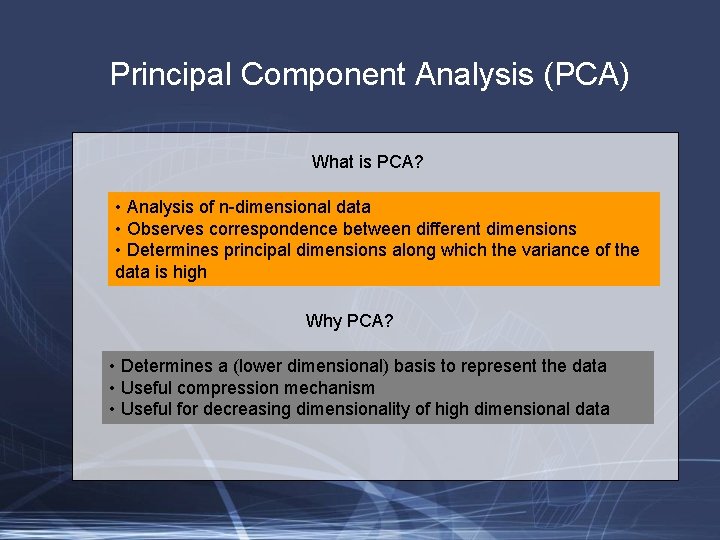
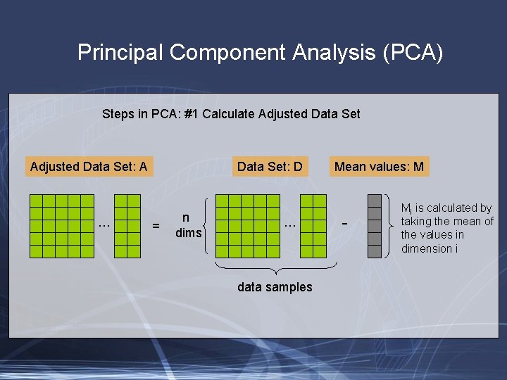
Principal Component Analysis (PCA) What is PCA? • Analysis of n-dimensional data • Observes correspondence between different dimensions • Determines principal dimensions along which the variance of the data is high Why PCA? • Determines a (lower dimensional) basis to represent the data • Useful compression mechanism • Useful for decreasing dimensionality of high dimensional data

Principal Component Analysis (PCA) Steps in PCA: #1 Calculate Adjusted Data Set: A … Data Set: D = n dims … data samples Mean values: M - Mi is calculated by taking the mean of the values in dimension i

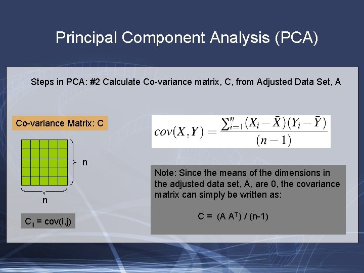
Principal Component Analysis (PCA) Steps in PCA: #2 Calculate Co-variance matrix, C, from Adjusted Data Set, A Co-variance Matrix: C n n Cij = cov(i, j) Note: Since the means of the dimensions in the adjusted data set, A, are 0, the covariance matrix can simply be written as: C = (A AT) / (n-1)

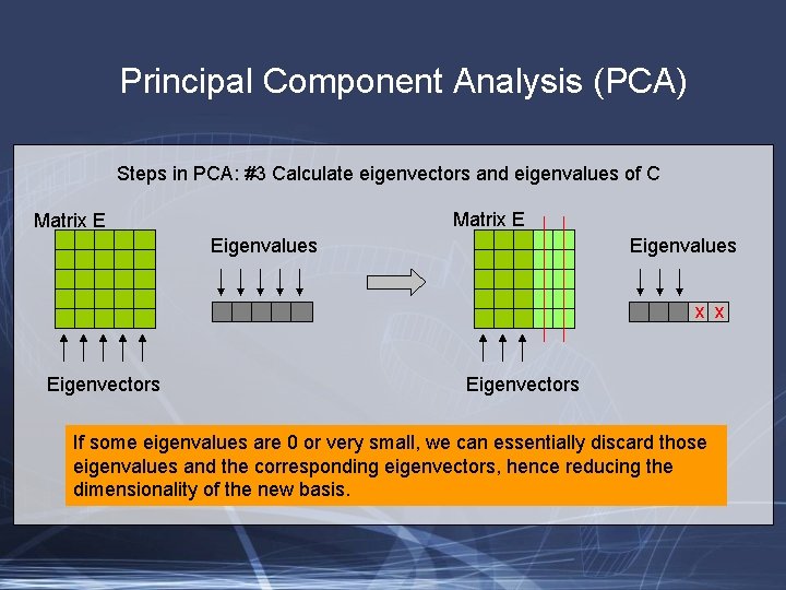
Principal Component Analysis (PCA) Steps in PCA: #3 Calculate eigenvectors and eigenvalues of C Matrix E Eigenvalues x x Eigenvectors If some eigenvalues are 0 or very small, we can essentially discard those eigenvalues and the corresponding eigenvectors, hence reducing the dimensionality of the new basis.

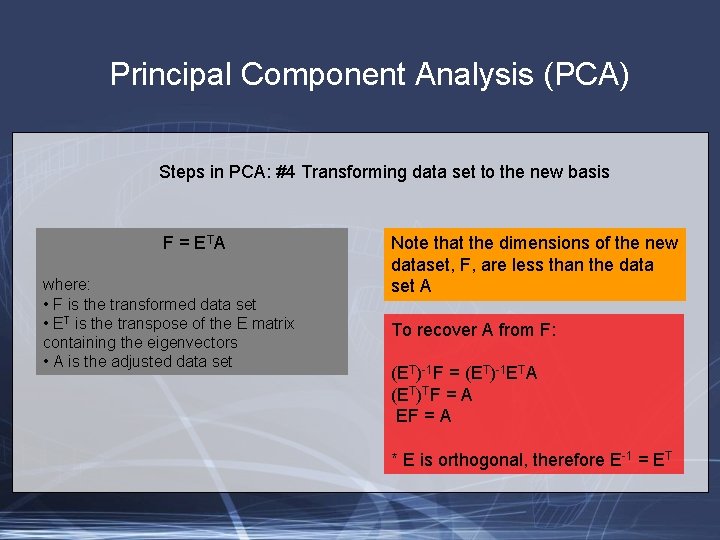
Principal Component Analysis (PCA) Steps in PCA: #4 Transforming data set to the new basis F = E TA where: • F is the transformed data set • ET is the transpose of the E matrix containing the eigenvectors • A is the adjusted data set Note that the dimensions of the new dataset, F, are less than the data set A To recover A from F: (ET)-1 F = (ET)-1 ETA (ET)TF = A EF = A * E is orthogonal, therefore E-1 = ET

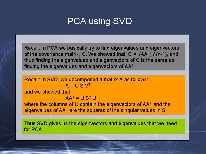
PCA using SVD Recall: In PCA we basically try to find eigenvalues and eigenvectors of the covariance matrix, C. We showed that C = (AAT) / (n-1), and thus finding the eigenvalues and eigenvectors of C is the same as finding the eigenvalues and eigenvectors of AAT Recall: In SVD, we decomposed a matrix A as follows: A = U S VT and we showed that: AAT = U S 2 UT where the columns of U contain the eigenvectors of AAT and the eigenvalues of AAT are the squares of the singular values in S Thus SVD gives us the eigenvectors and eigenvalues that we need for PCA

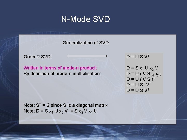
N-Mode SVD Generalization of SVD Order-2 SVD: D = U S VT Written in terms of mode-n product: By definition of mode-n multiplication: D = S x 1 U x 2 V D = U ( V S(2) )(1) D = U ( V S )T D = U S T VT D = U S VT Note: ST = S since S is a diagonal matrix Note: D = S x 1 U x 2 V = S x 2 V x 1 U

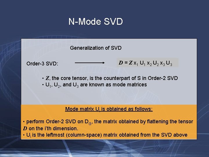
N-Mode SVD Generalization of SVD Order-3 SVD: D = Z x 1 U 1 x 2 U 2 x 3 U 3 • Z, the core tensor, is the counterpart of S in Order-2 SVD • U 1, U 2, and U 3 are known as mode matrices Mode matrix Ui is obtained as follows: • perform Order-2 SVD on D(i), the matrix obtained by flattening the tensor D on the i’th dimension. • Ui is the leftmost (column-space) matrix obtained from the SVD above

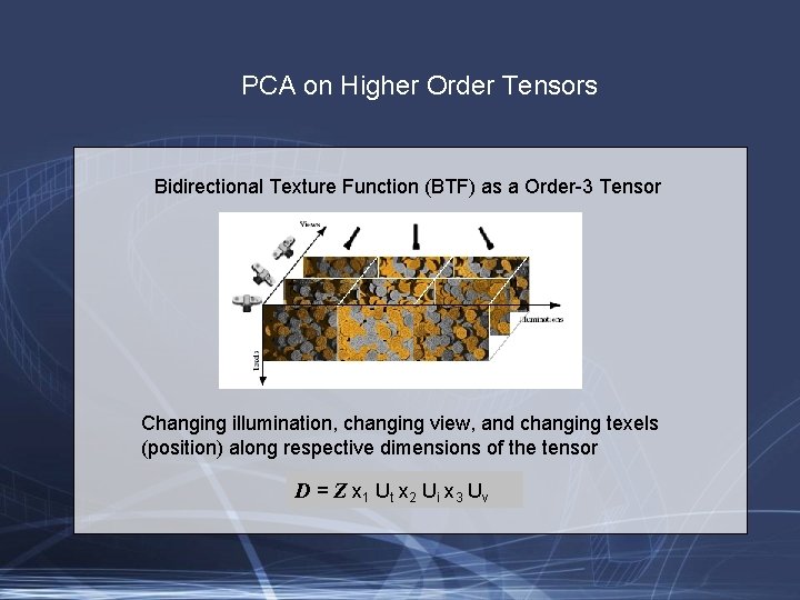
PCA on Higher Order Tensors Bidirectional Texture Function (BTF) as a Order-3 Tensor Changing illumination, changing view, and changing texels (position) along respective dimensions of the tensor D = Z x 1 Ut x 2 Ui x 3 Uv

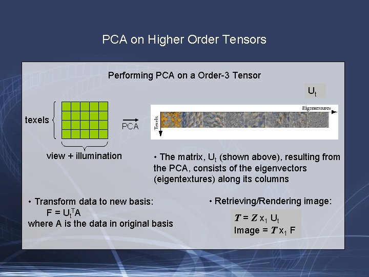
PCA on Higher Order Tensors Performing PCA on a Order-3 Tensor Ut texels view + illumination PCA • The matrix, Ut (shown above), resulting from the PCA, consists of the eigenvectors (eigentextures) along its columns • Transform data to new basis: F = Ut. TA where A is the data in original basis • Retrieving/Rendering image: T = Z x 1 Ut Image = T x 1 F

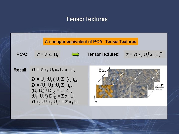
Tensor. Textures A cheaper equivalent of PCA: Tensor. Textures PCA: T = Z x 1 Ut Recall: D = Z x 1 Ut x 2 Ui x 3 Uv D = Uv (Ui ( Ut Z(1))(2))(3) D = (Uv Ui) (Ut Z(1))(2) (Uv Ui)-1 D(2) = Ut Z(1) (Ui. T Uv. T) D(3) = Z x 1 Ut D x 2 Ui. T x 3 Uv. T = Z x 1 Ut Tensor. Textures: T = D x 2 Ui. T x 3 Uv. T

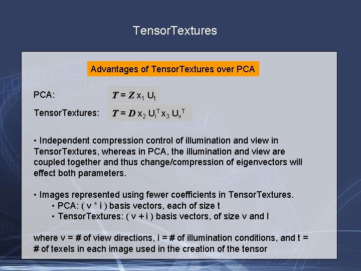
Tensor. Textures Advantages of Tensor. Textures over PCA: T = Z x 1 Ut Tensor. Textures: T = D x 2 Ui. T x 3 Uv. T • Independent compression control of illumination and view in Tensor. Textures, whereas in PCA, the illumination and view are coupled together and thus change/compression of eigenvectors will effect both parameters. • Images represented using fewer coefficients in Tensor. Textures. • PCA: ( v * i ) basis vectors, each of size t • Tensor. Textures: ( v + i ) basis vectors, of size v and I where v = # of view directions, i = # of illumination conditions, and t = # of texels in each image used in the creation of the tensor

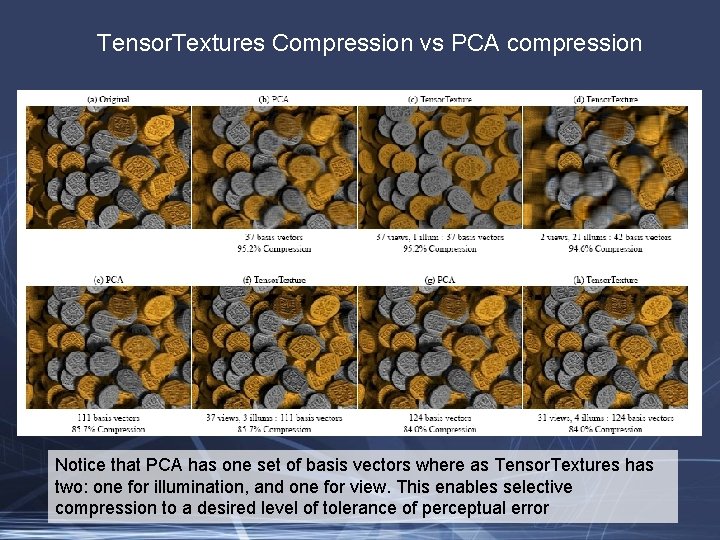
Tensor. Textures Compression vs PCA compression Notice that PCA has one set of basis vectors where as Tensor. Textures has two: one for illumination, and one for view. This enables selective compression to a desired level of tolerance of perceptual error