Temporal Plan Execution Dynamic Scheduling and Simple Temporal

Temporal Plan Execution: Dynamic Scheduling and Simple Temporal Networks Brian C. Williams 16. 412 J/6. 834 J December 2 nd, 2002 3/6/2021 1

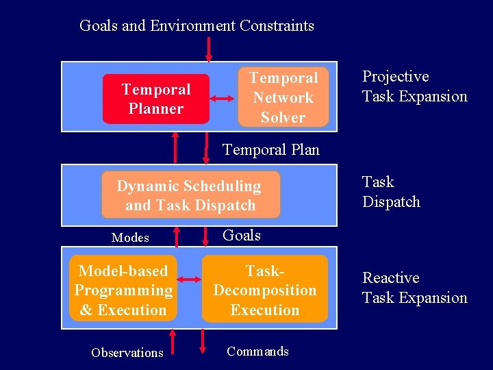
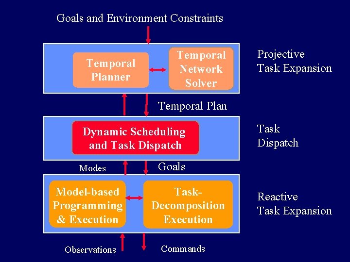
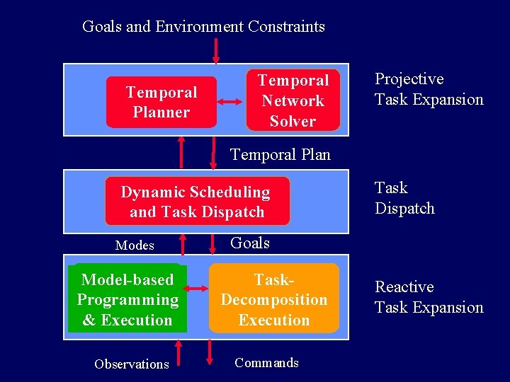
Goals and Environment Constraints Temporal Planner Temporal Network Solver Projective Task Expansion Temporal Plan Dynamic Scheduling and Task Dispatch Modes Model-based Programming & Execution Observations Task Dispatch Goals Task. Decomposition Execution Commands Reactive Task Expansion

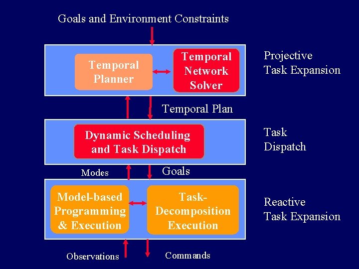
Goals and Environment Constraints Temporal Planner Temporal Network Solver Projective Task Expansion Temporal Plan Dynamic Scheduling and Task Dispatch Modes Model-based Programming & Execution Observations Task Dispatch Goals Task. Decomposition Execution Commands Reactive Task Expansion

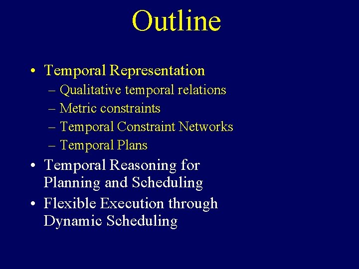
Outline • Temporal Representation – Qualitative temporal relations – Metric constraints – Temporal Constraint Networks – Temporal Plans • Temporal Reasoning for Planning and Scheduling • Flexible Execution through Dynamic Scheduling

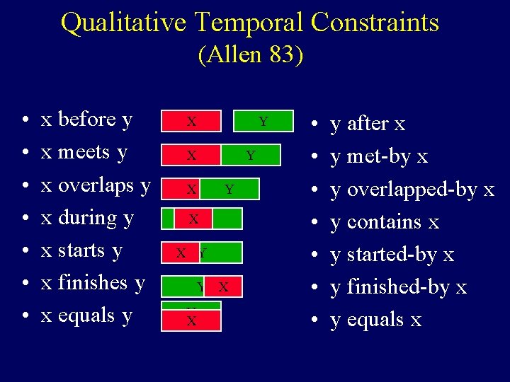
Qualitative Temporal Constraints (Allen 83) • • x before y x meets y x overlaps y x during y x starts y x finishes y x equals y X Y X Y XY X Y X • • y after x y met-by x y overlapped-by x y contains x y started-by x y finished-by x y equals x

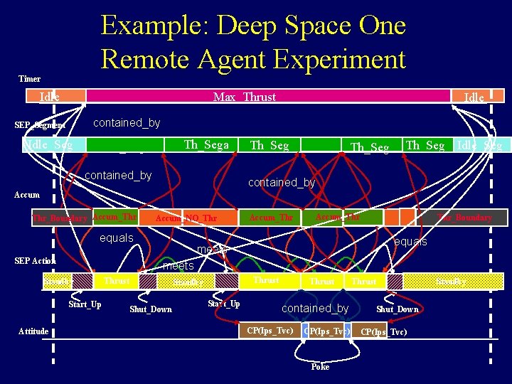
Example: Deep Space One Remote Agent Experiment Timer Max_Thrust Idle contained_by SEP_Segment Idle_Seg Th_Sega Th_Seg contained_by Th_Seg Idle_Seg contained_by Accum Thr_Boundary Accum_Thr Accum_NO_Thr equals SEP Action Accum_Thr Thr_Boundary equals meets Standby Start_Up Attitude Accum_Thr Thrust Standby Shut_Down Start_Up Thrust contained_by CP(Ips_Tvc) Poke Thrust Shut_Down CP(Ips_Tvc) Standby

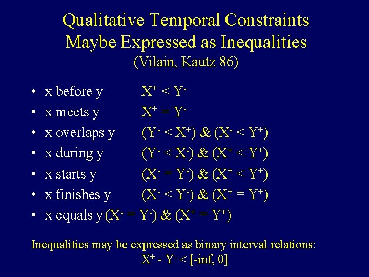
Qualitative Temporal Constraints Maybe Expressed as Inequalities (Vilain, Kautz 86) • • x before y X+ < Y x meets y X+ = Y x overlaps y (Y- < X+) & (X- < Y+) x during y (Y- < X-) & (X+ < Y+) x starts y (X- = Y-) & (X+ < Y+) x finishes y (X- < Y-) & (X+ = Y+) x equals y (X- = Y-) & (X+ = Y+) Inequalities may be expressed as binary interval relations: X+ - Y- < [-inf, 0]

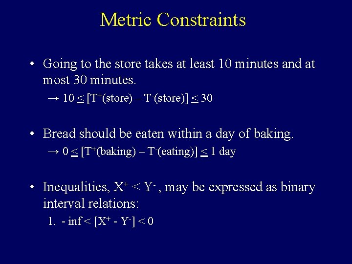
Metric Constraints • Going to the store takes at least 10 minutes and at most 30 minutes. → 10 < [T+(store) – T-(store)] < 30 • Bread should be eaten within a day of baking. → 0 < [T+(baking) – T-(eating)] < 1 day • Inequalities, X+ < Y- , may be expressed as binary interval relations: 1. - inf < [X+ - Y-] < 0

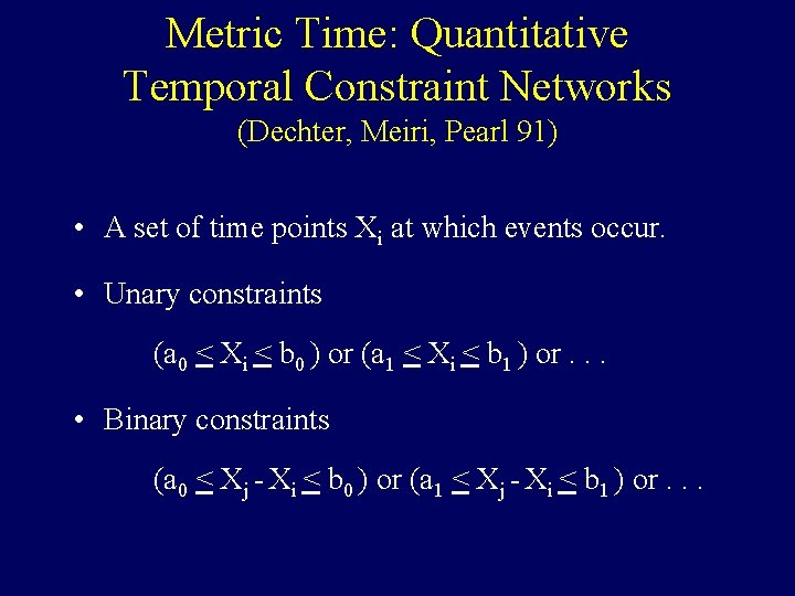
Metric Time: Quantitative Temporal Constraint Networks (Dechter, Meiri, Pearl 91) • A set of time points Xi at which events occur. • Unary constraints (a 0 < Xi < b 0 ) or (a 1 < Xi < b 1 ) or. . . • Binary constraints (a 0 < Xj - Xi < b 0 ) or (a 1 < Xj - Xi < b 1 ) or. . .

TCSP Are Visualized Using Directed Constraint Graphs 0 [10, 20] 1 [30, 40] [60, inf] 3 [10, 20] 2 [20, 30] [40, 50] [60, 70] 4

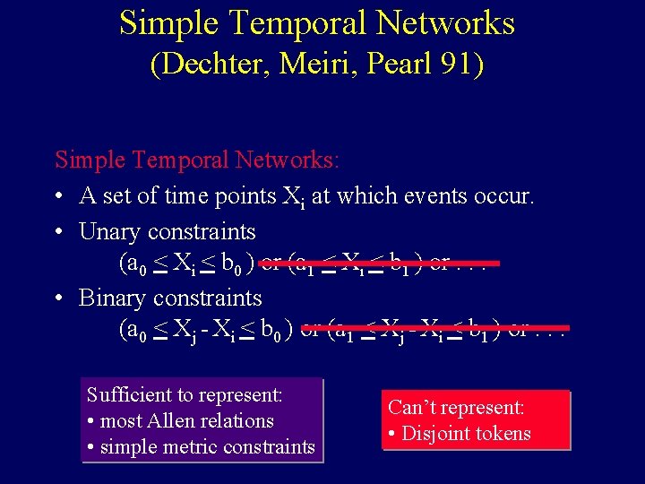
Simple Temporal Networks (Dechter, Meiri, Pearl 91) Simple Temporal Networks: • A set of time points Xi at which events occur. • Unary constraints (a 0 < Xi < b 0 ) or (a 1 < Xi < b 1 ) or. . . • Binary constraints (a 0 < Xj - Xi < b 0 ) or (a 1 < Xj - Xi < b 1 ) or. . . Sufficient to represent: • most Allen relations • simple metric constraints Can’t represent: • Disjoint tokens

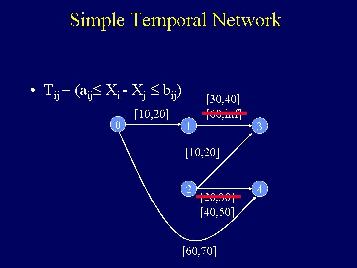
Simple Temporal Network • Tij = (aij£ Xi - Xj £ bij) 0 [10, 20] 1 [30, 40] [60, inf] 3 [10, 20] 2 [20, 30] [40, 50] [60, 70] 4

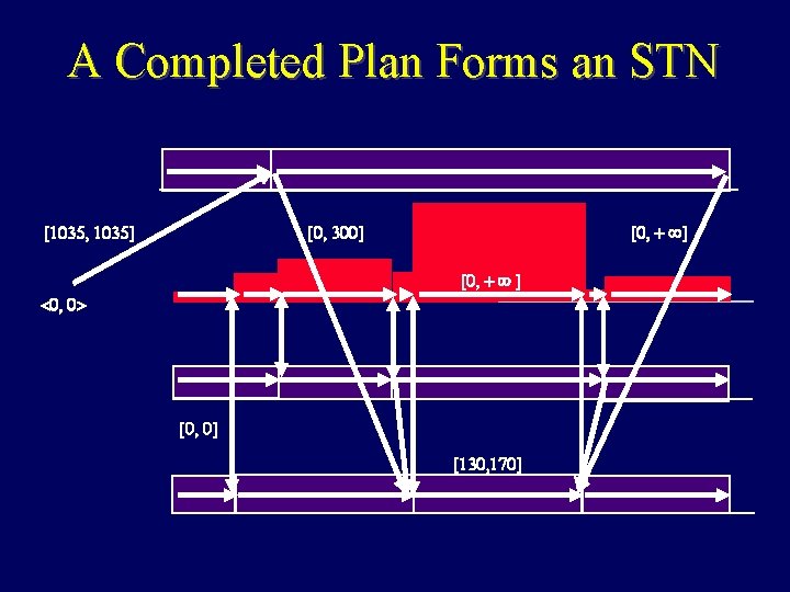
A Completed Plan Forms an STN

Outline • Temporal Representation • Temporal Reasoning for Planning and Scheduling – TCSP Queries – Induced Constraints – Plan Consistency – Static Scheduling • Flexible Execution through Dynamic Scheduling

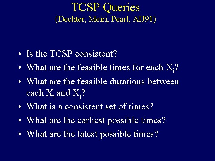
TCSP Queries (Dechter, Meiri, Pearl, AIJ 91) • Is the TCSP consistent? • What are the feasible times for each Xi? • What are the feasible durations between each Xi and Xj? • What is a consistent set of times? • What are the earliest possible times? • What are the latest possible times?

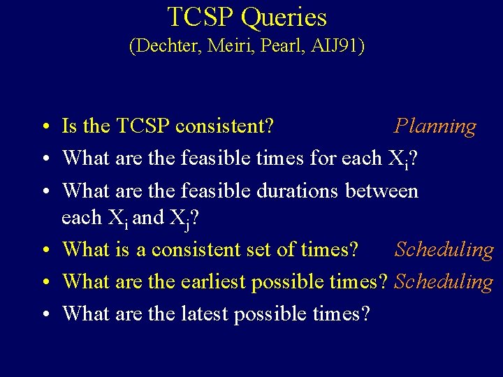
TCSP Queries (Dechter, Meiri, Pearl, AIJ 91) • Is the TCSP consistent? Planning • What are the feasible times for each Xi? • What are the feasible durations between each Xi and Xj? • What is a consistent set of times? Scheduling • What are the earliest possible times? Scheduling • What are the latest possible times?

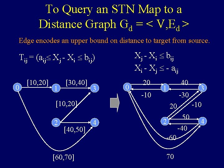
To Query an STN Map to a Distance Graph Gd = < V, Ed > Edge encodes an upper bound on distance to target from source. Xj - Xi £ bij Xi - Xj £ - aij Tij = (aij£ Xj - Xi £ bij) 0 [10, 20] 1 [30, 40] 3 0 20 -10 1 [10, 20] 2 [40, 50] [60, 70] 40 -30 -10 20 4 2 -60 70 3 50 -40 4

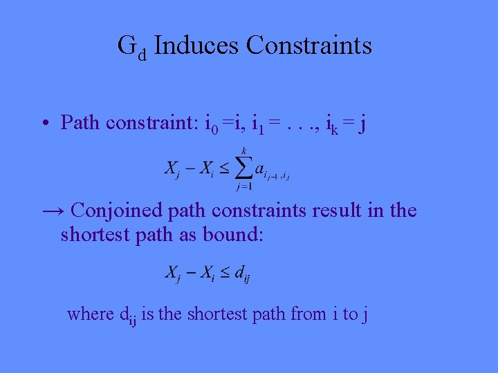
Gd Induces Constraints • Path constraint: i 0 =i, i 1 =. . . , ik = j → Conjoined path constraints result in the shortest path as bound: where dij is the shortest path from i to j

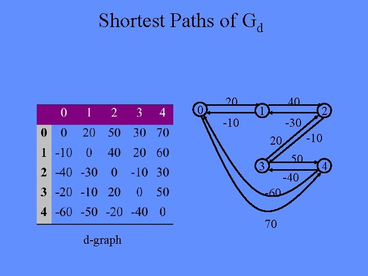
Shortest Paths of Gd 0 20 -10 40 1 -30 -10 20 3 -60 70 d-graph 2 50 -40 4

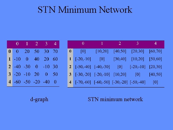
STN Minimum Network d-graph STN minimum network

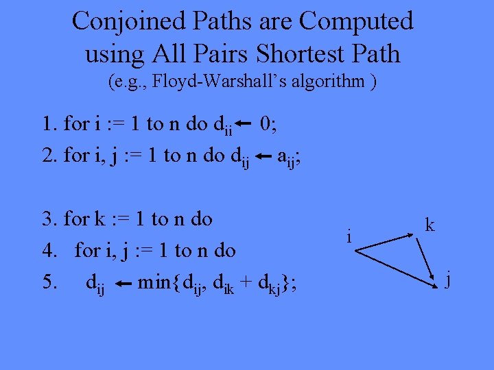
Conjoined Paths are Computed using All Pairs Shortest Path (e. g. , Floyd-Warshall’s algorithm ) 1. for i : = 1 to n do dii 0; 2. for i, j : = 1 to n do dij aij; 3. for k : = 1 to n do 4. for i, j : = 1 to n do 5. dij min{dij, dik + dkj}; i k j

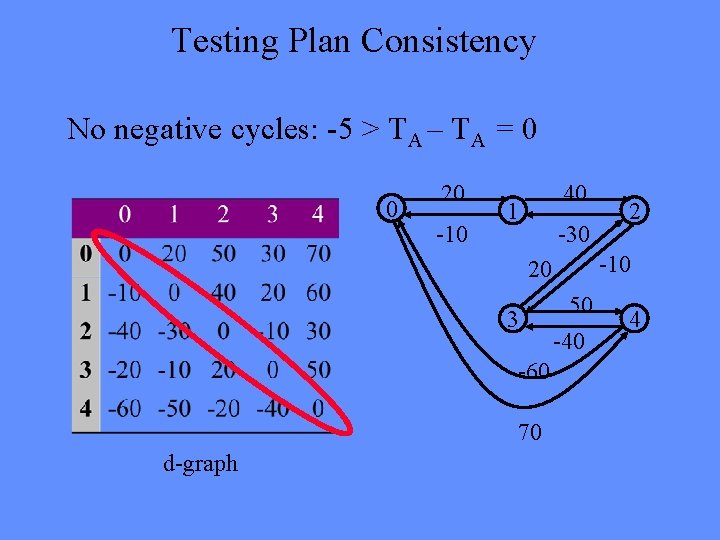
Testing Plan Consistency No negative cycles: -5 > TA – TA = 0 0 20 -10 40 1 -30 -10 20 3 -60 70 d-graph 2 50 -40 4

Scheduling: Feasible Values Latest Times • X 1 in [10, 20] • X 2 in [40, 50] • X 3 in [20, 30] • X 4 in [60, 70] Earliest Times d-graph

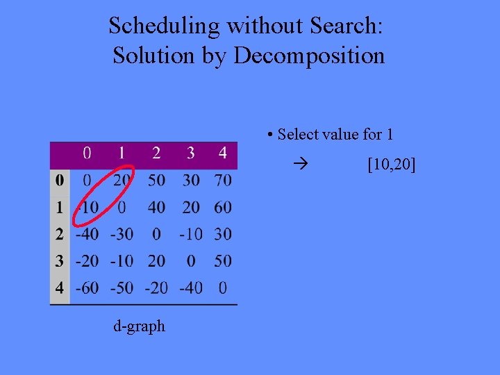
Scheduling without Search: Solution by Decomposition • Select value for 1 à 15 d-graph [10, 20]

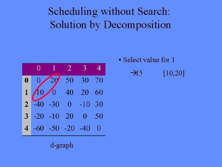
Scheduling without Search: Solution by Decomposition • Select value for 1 à 15 d-graph [10, 20]

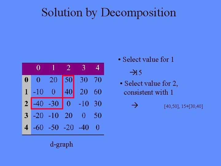
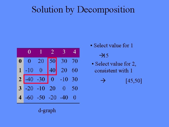
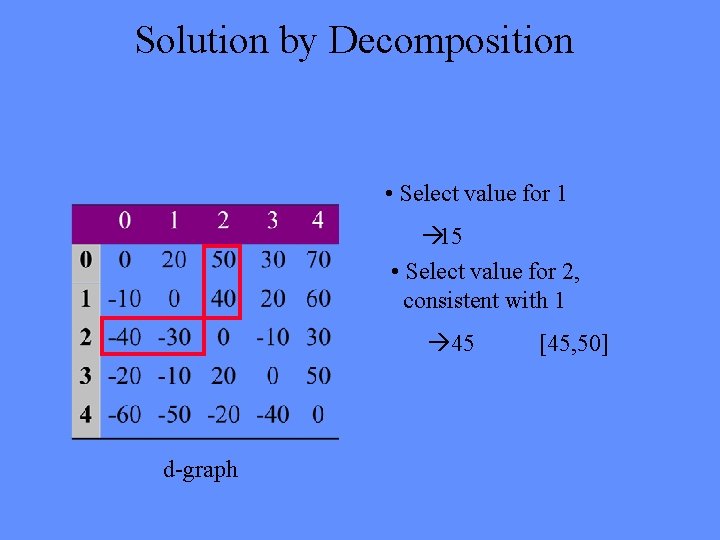
Solution by Decomposition • Select value for 1 à 15 • Select value for 2, consistent with 1 à 45 d-graph [40, 50], 15+[30, 40]

Solution by Decomposition • Select value for 1 à 15 • Select value for 2, consistent with 1 à 45 d-graph [45, 50]

Solution by Decomposition • Select value for 1 à 15 • Select value for 2, consistent with 1 à 45 d-graph [45, 50]

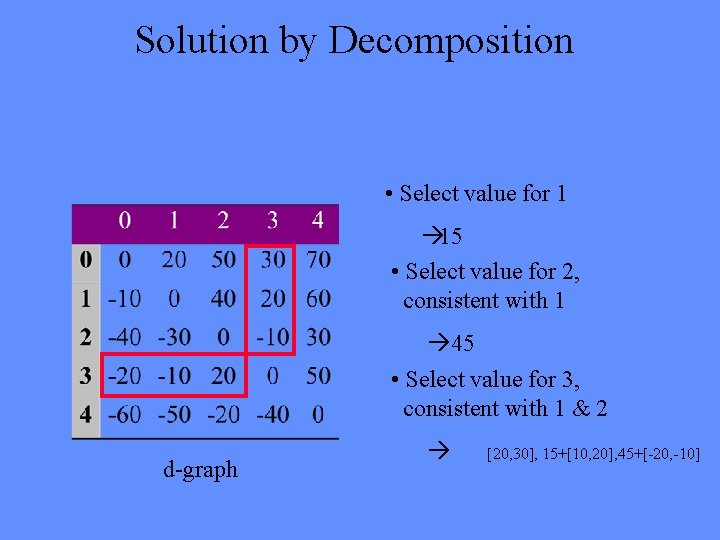
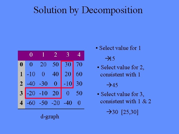
Solution by Decomposition • Select value for 1 à 15 • Select value for 2, consistent with 1 à 45 • Select value for 3, consistent with 1 & 2 d-graph à 30 [20, 30], 15+[10, 20], 45+[-20, -10]

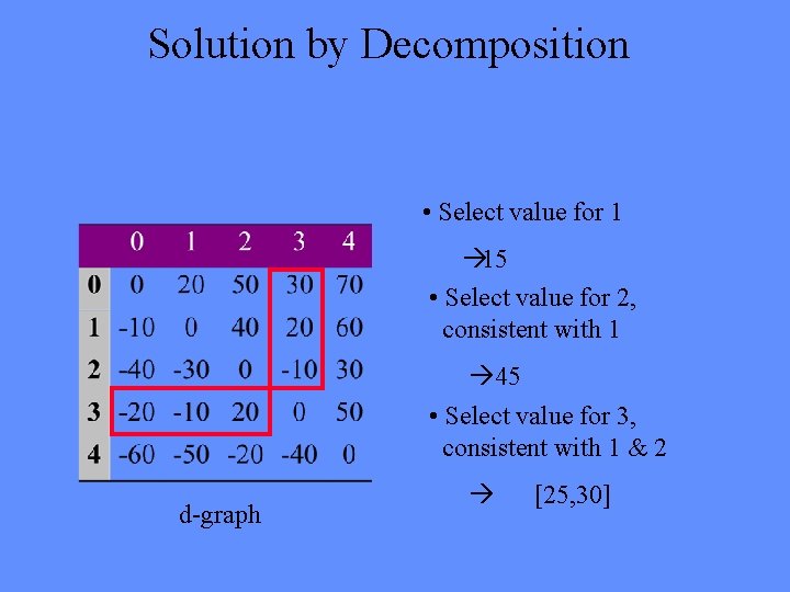
Solution by Decomposition • Select value for 1 à 15 • Select value for 2, consistent with 1 à 45 • Select value for 3, consistent with 1 & 2 d-graph à 30 [25, 30]

Solution by Decomposition • Select value for 1 à 15 • Select value for 2, consistent with 1 à 45 • Select value for 3, consistent with 1 & 2 d-graph à 30 [25, 30]

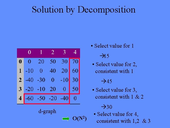
Solution by Decomposition • Select value for 1 à 15 • Select value for 2, consistent with 1 à 45 • Select value for 3, consistent with 1 & 2 d-graph O(N 2) à 30 • Select value for 4, consistent with 1, 2 & 3

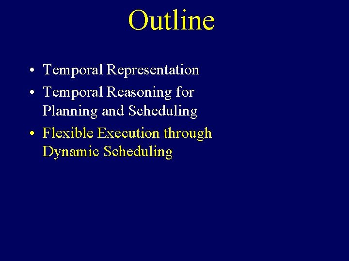
Outline • Temporal Representation • Temporal Reasoning for Planning and Scheduling • Flexible Execution through Dynamic Scheduling

Goals and Environment Constraints Temporal Planner Temporal Network Solver Projective Task Expansion Temporal Plan Dynamic Scheduling and Task Dispatch Modes Model-based Programming & Execution Observations Task Dispatch Goals Task. Decomposition Execution Commands Reactive Task Expansion

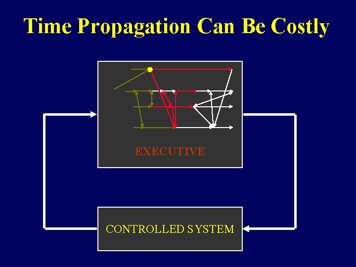
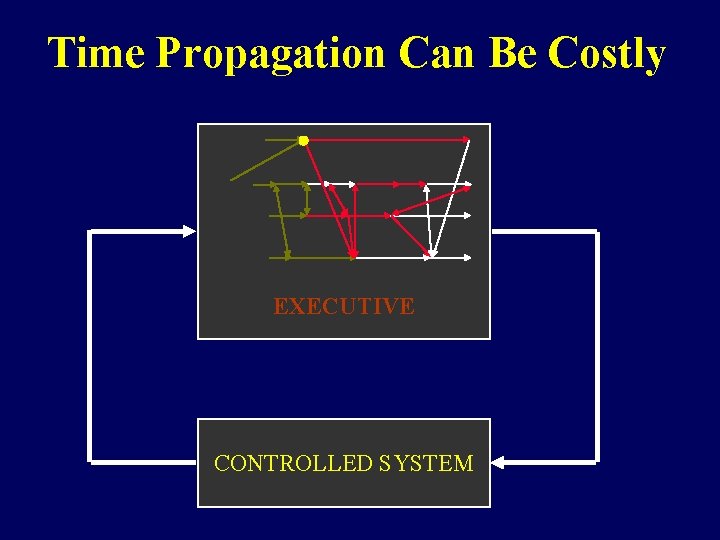
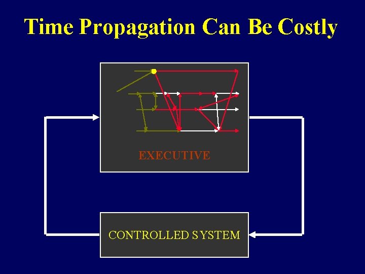
Executing Flexible Temporal Plans [Muscettola, Morris, Pell et al. ] Handling delays and fluctuations in task duration: • Least commitment temporal plans leave room to adapt EXECUTIVE CONTROLLED SYSTEM • flexible execution adapts through dynamic scheduling • Assigns time to event when executed.

Issues in Flexible Execution 1. How do we minimize execution latency? 2. How do we schedule at execution time?

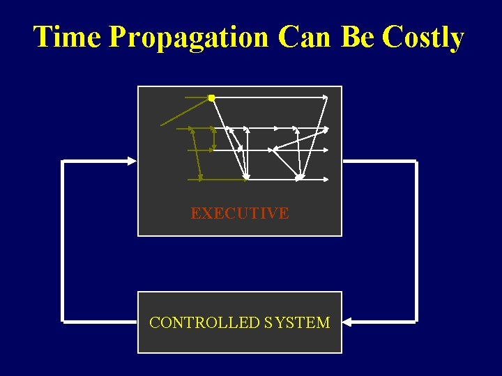
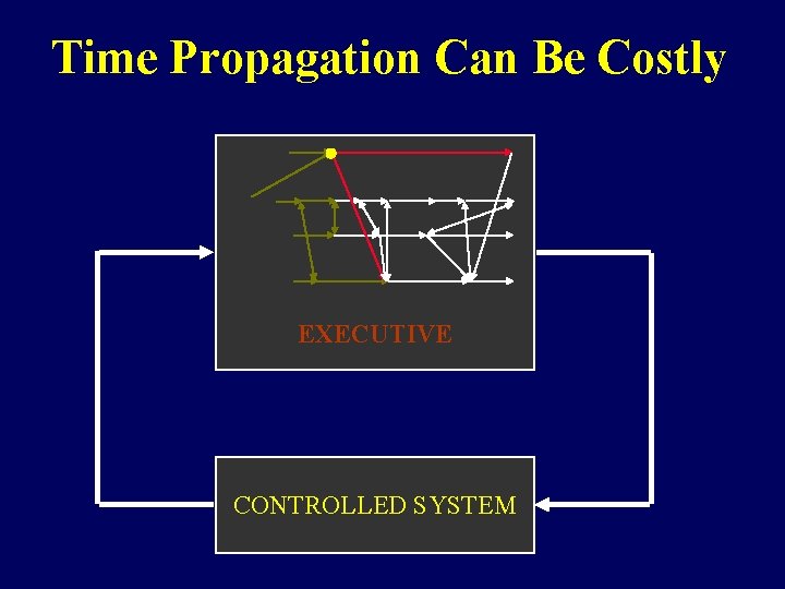
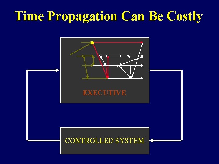
Time Propagation Can Be Costly EXECUTIVE CONTROLLED SYSTEM

Time Propagation Can Be Costly EXECUTIVE CONTROLLED SYSTEM

Time Propagation Can Be Costly EXECUTIVE CONTROLLED SYSTEM

Time Propagation Can Be Costly EXECUTIVE CONTROLLED SYSTEM

Time Propagation Can Be Costly EXECUTIVE CONTROLLED SYSTEM

Time Propagation Can Be Costly EXECUTIVE CONTROLLED SYSTEM

Issues in Flexible Execution 1. How do we minimize execution latency? è Propagate through a small set of neighboring constraints. 2. How do we schedule at execution time?

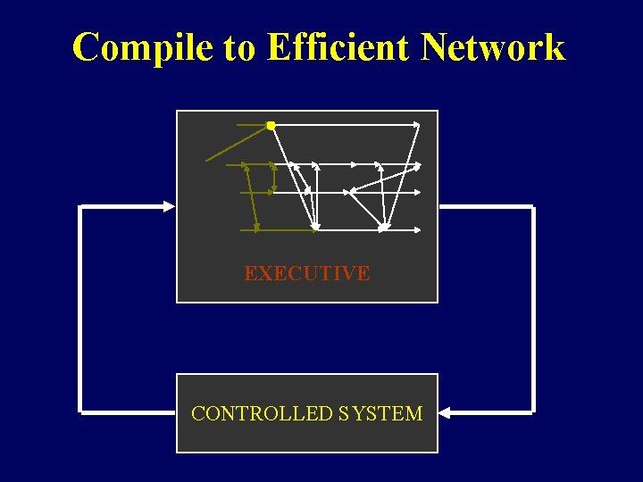
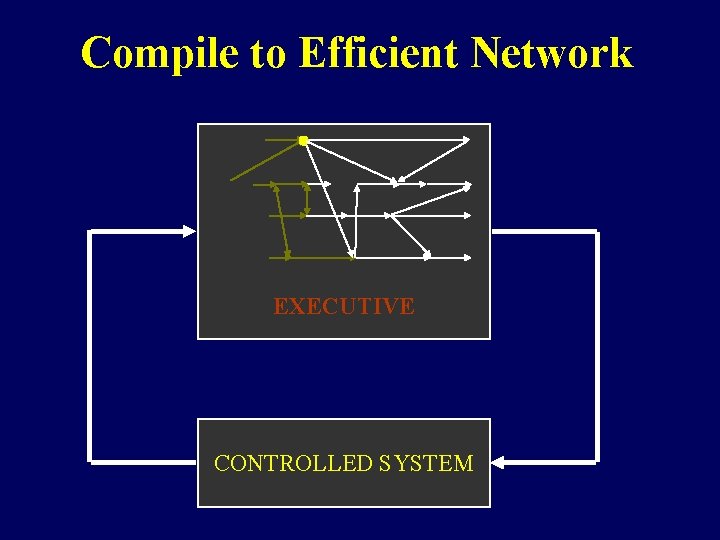
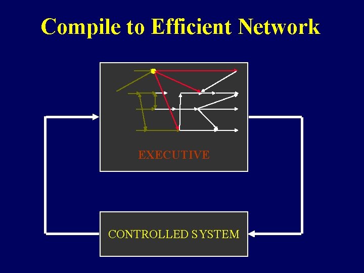
Compile to Efficient Network EXECUTIVE CONTROLLED SYSTEM

Compile to Efficient Network EXECUTIVE CONTROLLED SYSTEM

Compile to Efficient Network EXECUTIVE CONTROLLED SYSTEM

Issues in Flexible Execution 1. How do we minimize execution latency? è Propagate through a small set of neighboring constraints. 2. How do we schedule at execution time?

Issues in Flexible Execution 1. How do we minimize execution latency? è Propagate through a small set of neighboring constraints. 2. How do we schedule at execution time? è Through decomposition?

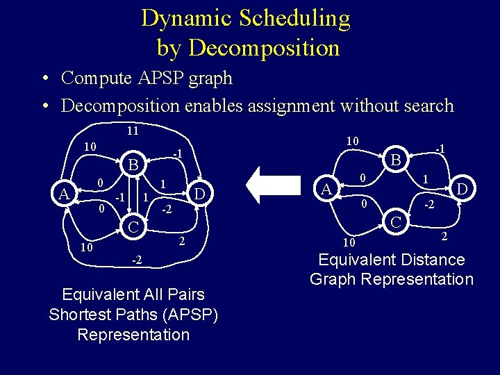
Dynamic Scheduling by Decomposition [0, 10] B 10 [-1, 1] A B D [0, 10] C -1 A 1 0 -2 C [-2, 2] 10 Simple Example 0 D 2 Equivalent Distance Graph Representation

Dynamic Scheduling by Decomposition • Compute APSP graph • Decomposition enables assignment without search 11 10 -1 B 0 A 0 -1 1 C 10 10 1 B D -2 -1 A 0 1 0 -2 C 2 -2 Equivalent All Pairs Shortest Paths (APSP) Representation 10 D 2 Equivalent Distance Graph Representation

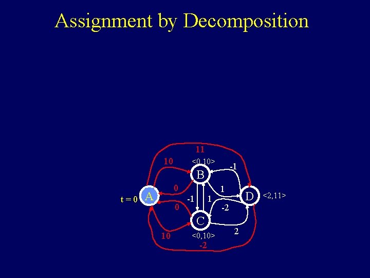
Assignment by Decomposition 11 10 <0, 10> -1 B t=0 0 A 0 -1 1 C 10 <0, 10> -2 1 D -2 2 <2, 11>

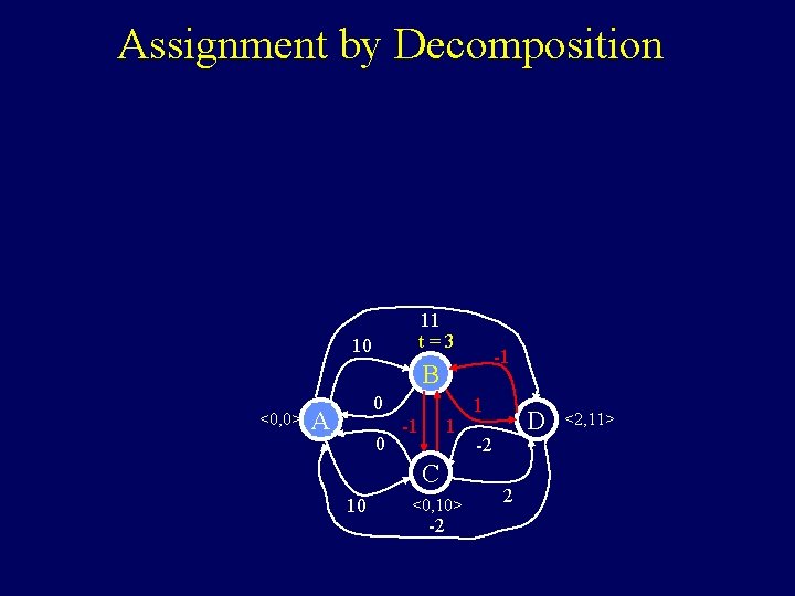
Assignment by Decomposition 11 t=3 10 -1 B <0, 0> 0 A 0 -1 1 C 10 <0, 10> -2 1 D -2 2 <2, 11>

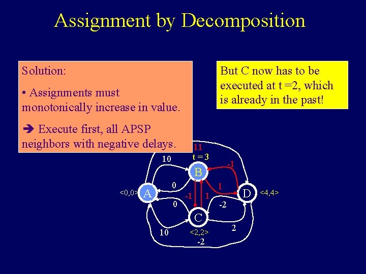
Assignment by Decomposition Solution: But C now has to be executed at t =2, which is already in the past! • Assignments must monotonically increase in value. è Execute first, all APSP neighbors with negative delays. 10 11 t=3 -1 B <0, 0> 0 A 0 -1 1 C 10 <2, 2> -2 1 D -2 2 <4, 4>

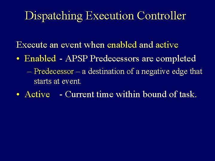
Dispatching Execution Controller Execute an event when enabled and active • Enabled - APSP Predecessors are completed – Predecessor – a destination of a negative edge that starts at event. • Active - Current time within bound of task.

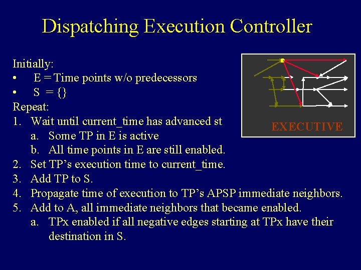
Dispatching Execution Controller Initially: • E = Time points w/o predecessors • S = {} Repeat: 1. Wait until current_time has advanced st EXECUTIVE a. Some TP in E is active b. All time points in E are still enabled. 2. Set TP’s execution time to current_time. 3. Add TP to S. 4. Propagate time of execution to TP’s APSP immediate neighbors. 5. Add to A, all immediate neighbors that became enabled. a. TPx enabled if all negative edges starting at TPx have their destination in S.

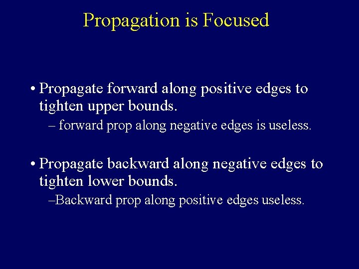
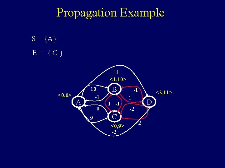
Propagation is Focused • Propagate forward along positive edges to tighten upper bounds. – forward prop along negative edges is useless. • Propagate backward along negative edges to tighten lower bounds. –Backward prop along positive edges useless.

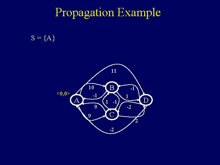
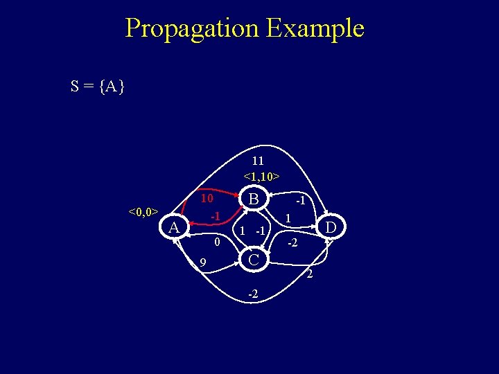
Propagation Example S = {A} 11 <0, 0> A 10 -1 0 9 B 1 -1 C -2 -1 1 D -2 2

Propagation Example S = {A} 11 <1, 10> <0, 0> A 10 -1 0 9 B 1 -1 C -2 -1 1 D -2 2

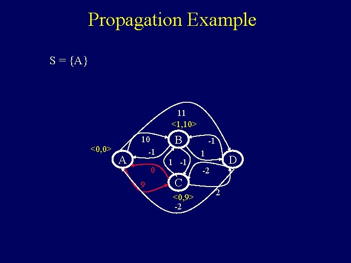
Propagation Example S = {A} 11 <1, 10> <0, 0> A 10 -1 0 9 B 1 -1 C <0, 9> -2 -1 1 D -2 2

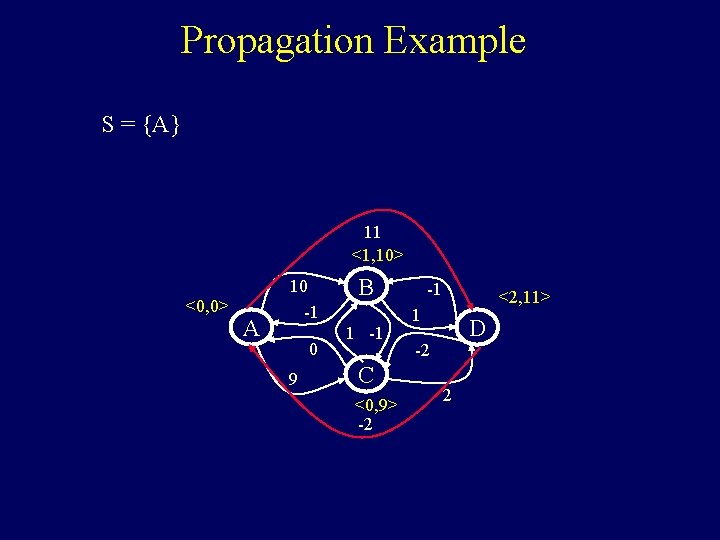
Propagation Example S = {A} 11 <1, 10> <0, 0> A 10 -1 0 9 B 1 -1 C <0, 9> -2 -1 <2, 11> 1 D -2 2

Propagation Example S = {A} E= {C} 11 <1, 10> <0, 0> A 10 -1 0 9 B 1 -1 C <0, 9> -2 -1 <2, 11> 1 D -2 2

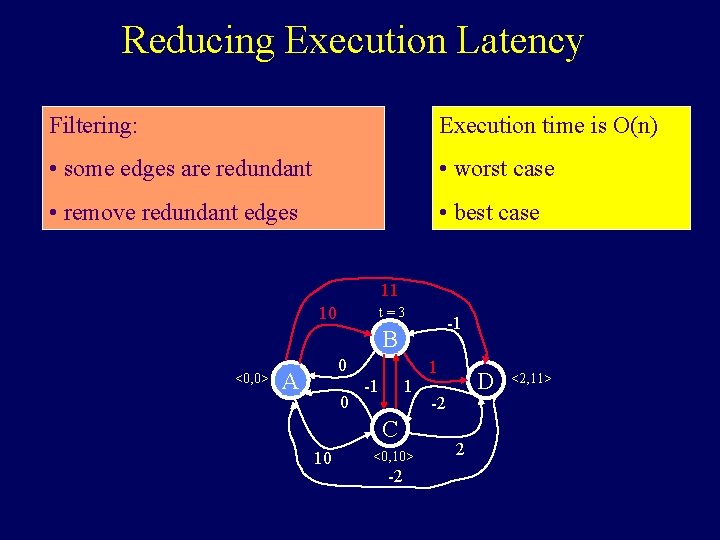
Reducing Execution Latency Filtering: Execution time is O(n) • some edges are redundant • worst case • remove redundant edges • best case 11 10 t=3 -1 B <0, 0> 0 A 0 -1 1 C 10 <0, 10> -2 1 D -2 2 <2, 11>

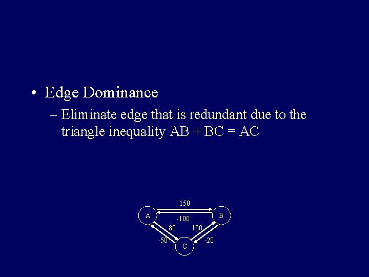
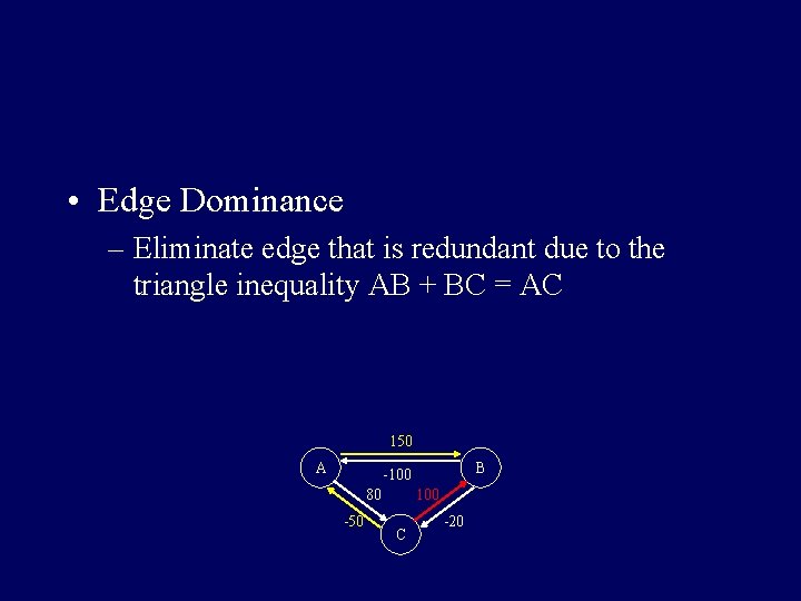
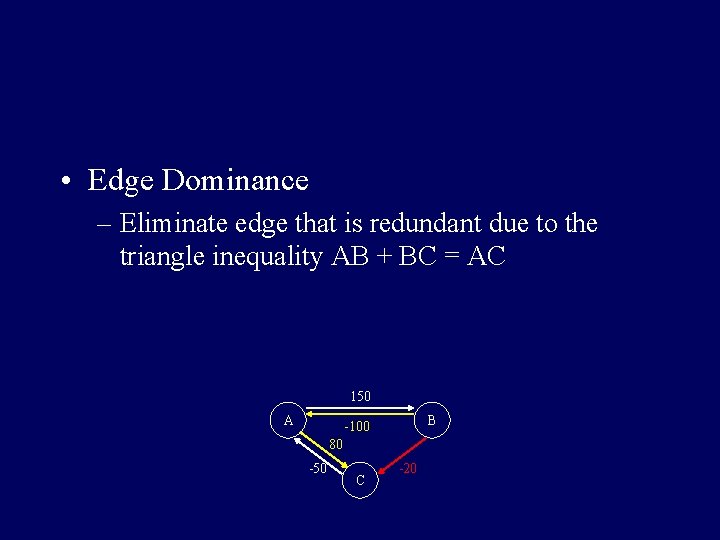
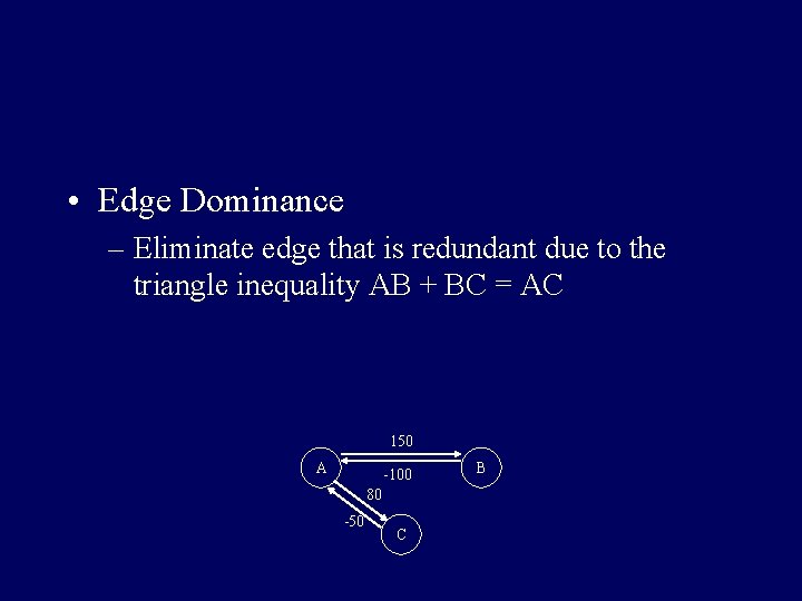
• Edge Dominance – Eliminate edge that is redundant due to the triangle inequality AB + BC = AC 150 A B -100 80 -50 100 C -20

• Edge Dominance – Eliminate edge that is redundant due to the triangle inequality AB + BC = AC 150 A B -100 80 -50 100 C -20

• Edge Dominance – Eliminate edge that is redundant due to the triangle inequality AB + BC = AC 150 A B -100 80 -50 C -20

• Edge Dominance – Eliminate edge that is redundant due to the triangle inequality AB + BC = AC 150 A -100 80 -50 C B

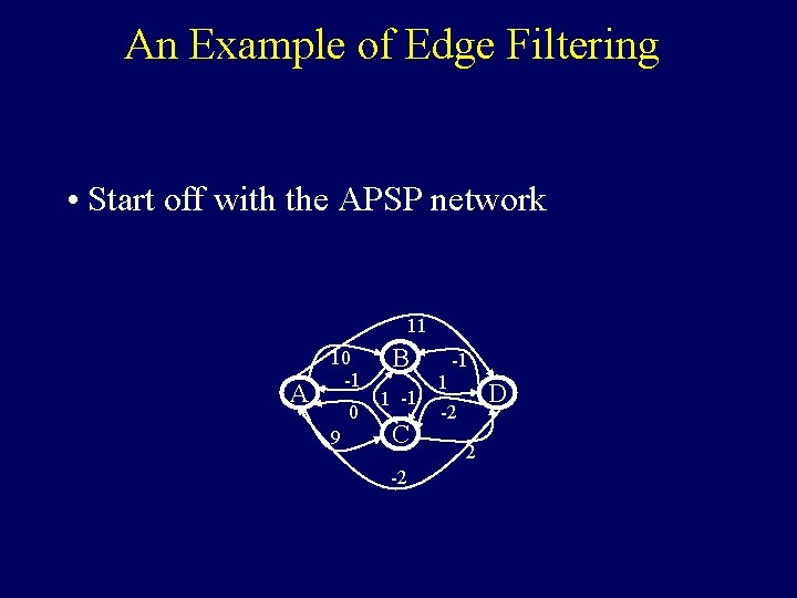
An Example of Edge Filtering • Start off with the APSP network 11 A 10 -1 0 9 B 1 -1 C -2 1 -1 D -2 2

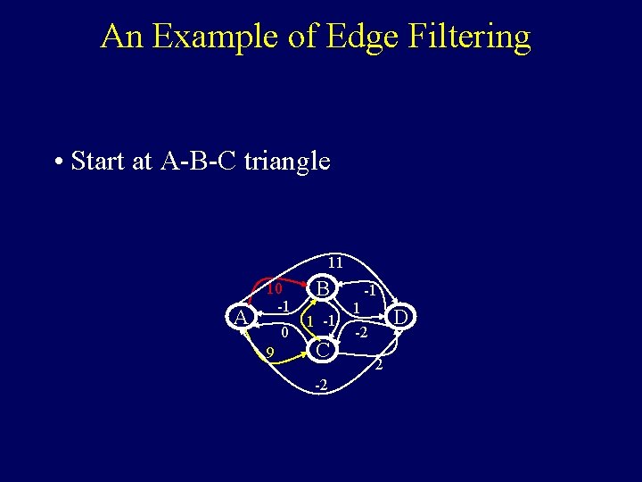
An Example of Edge Filtering • Start at A-B-C triangle 11 A 10 -1 0 9 B 1 -1 C -2 1 -1 D -2 2

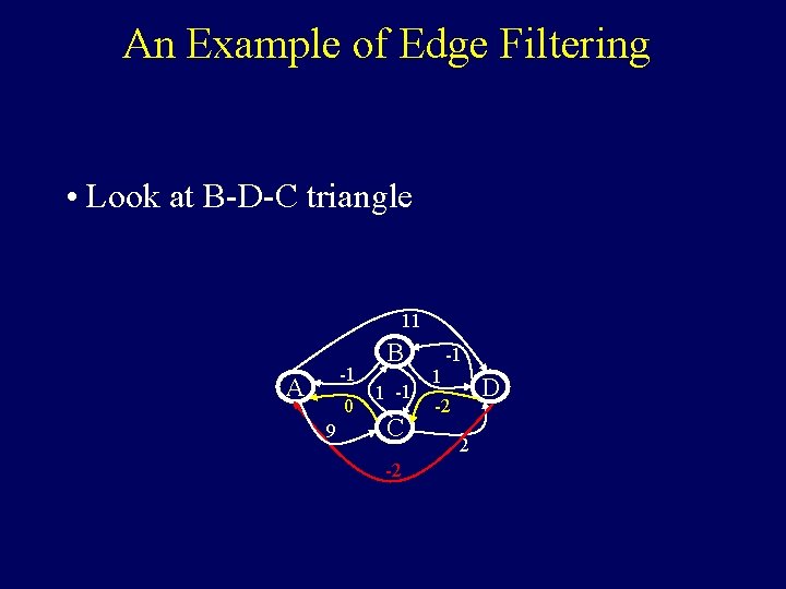
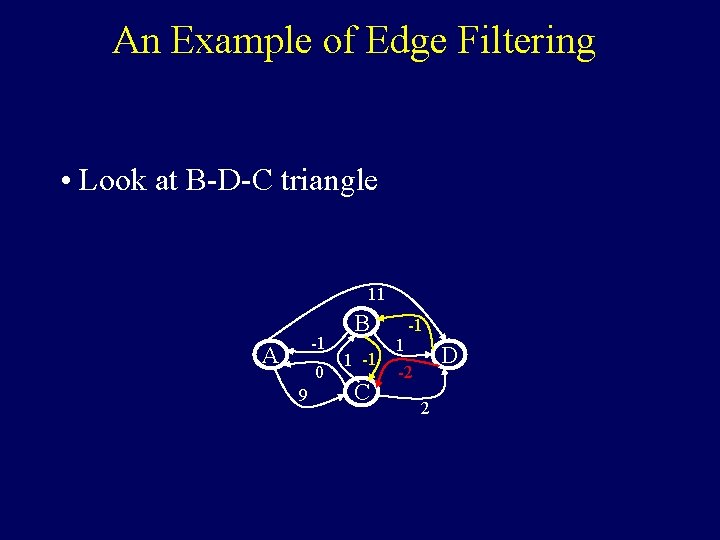
An Example of Edge Filtering • Look at B-D-C triangle 11 -1 A 0 9 B 1 -1 C -2 1 -1 D -2 2

An Example of Edge Filtering • Look at B-D-C triangle 11 -1 A 0 9 B 1 -1 C 1 -1 D -2 2

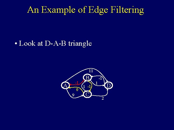
An Example of Edge Filtering • Look at D-A-B triangle 11 -1 A 0 9 B 1 -1 C 1 -1 D 2

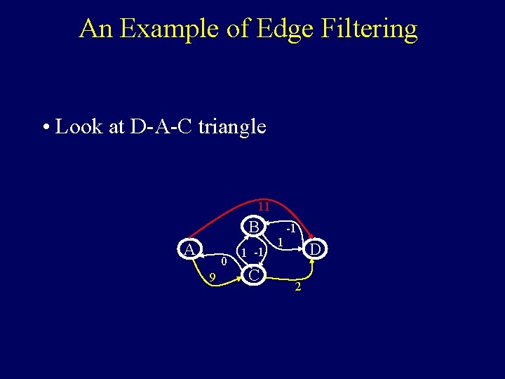
An Example of Edge Filtering • Look at D-A-C triangle 11 B A 0 9 1 -1 C 1 -1 D 2

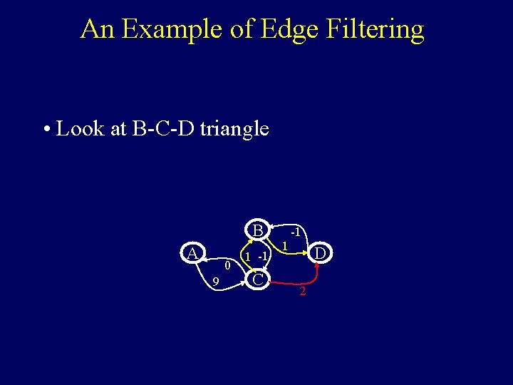
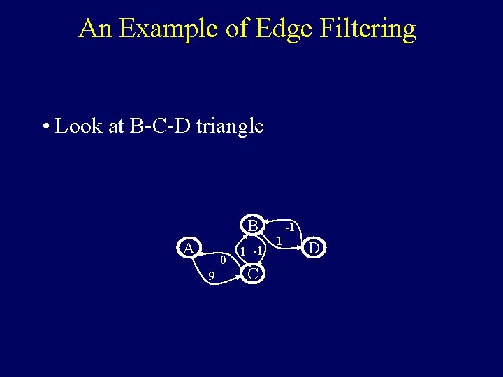
An Example of Edge Filtering • Look at B-C-D triangle B A 0 9 1 -1 C 1 -1 D 2

An Example of Edge Filtering • Look at B-C-D triangle B A 0 9 1 -1 C 1 -1 D

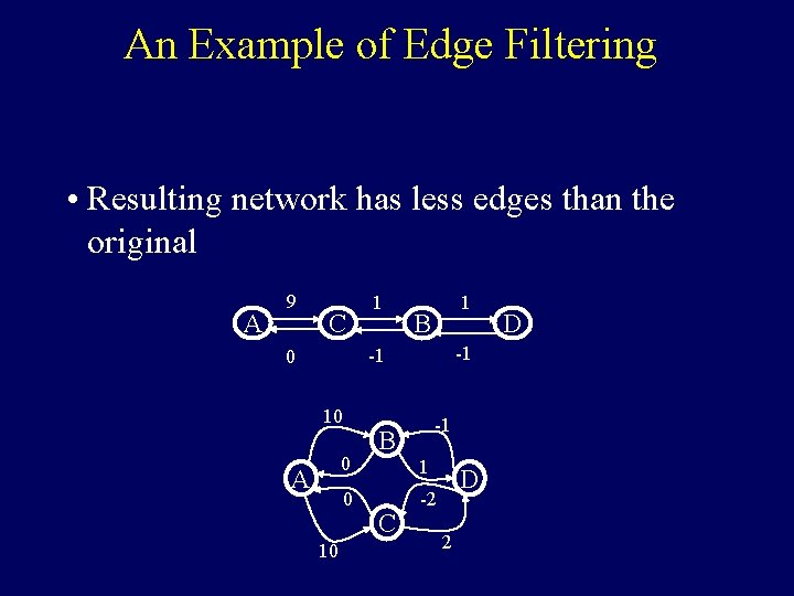
An Example of Edge Filtering • Resulting network has less edges than the original A 9 C 1 1 B -1 -1 0 10 0 A 0 10 -1 B 1 C D -2 2 D

Avoiding Intermediate Graph Explosion Problem: • APSP consumes O(n 2) space. Solution: • Interleave process of APSP construction with edge elimination – Never have to build whole APSP graph

Goals and Environment Constraints Temporal Planner Temporal Network Solver Projective Task Expansion Temporal Plan Dynamic Scheduling and Task Dispatch Modes Model-based Programming & Execution Observations Task Dispatch Goals Task. Decomposition Execution Commands Reactive Task Expansion